Understanding the Macroeconomic Implications of Heterogeneity

In the past decade, the widespread availability of large household- and firm-level datasets has sparked a “micro data” revolution in macroeconomics. Our research tries to understand the macroeconomic implications of this microeconomic heterogeneity by answering two key questions. First, what features of the micro data are most informative about macroeconomic outcomes? In particular, when can we find micro-sufficient statistics for these macro effects? Second, how can we make sure that our models match these moments while continuing to fit the macroeconomic data well?

In the traditional analysis of fiscal policy based on the “Keynesian cross,” the aggregate effects of government spending or transfers are determined by the marginal propensity to consume (MPC). For instance, the multiplier giving the effect of a fiscal transfer on GDP is MPC/(1 – MPC), which includes both the direct effect of the transfer on spending and the equilibrium effect from higher aggregate income. This classic result has made the MPC a very popular object to measure, both at the aggregate and at the individual level. 

However, as pointed out by Milton Friedman and Franco Modigliani in the 1950s and 1960s, the MPC concept has important limitations in a dynamic context. Since consumers are forward-looking, income today affects consumption in the future via savings, and anticipation of future income affects consumption today. In modern dynamic models, therefore, understanding consumption behavior requires going beyond the MPC to study the entire impulse response of consumption to income, which we call the “intertemporal marginal propensity to consume,” or iMPC.¹

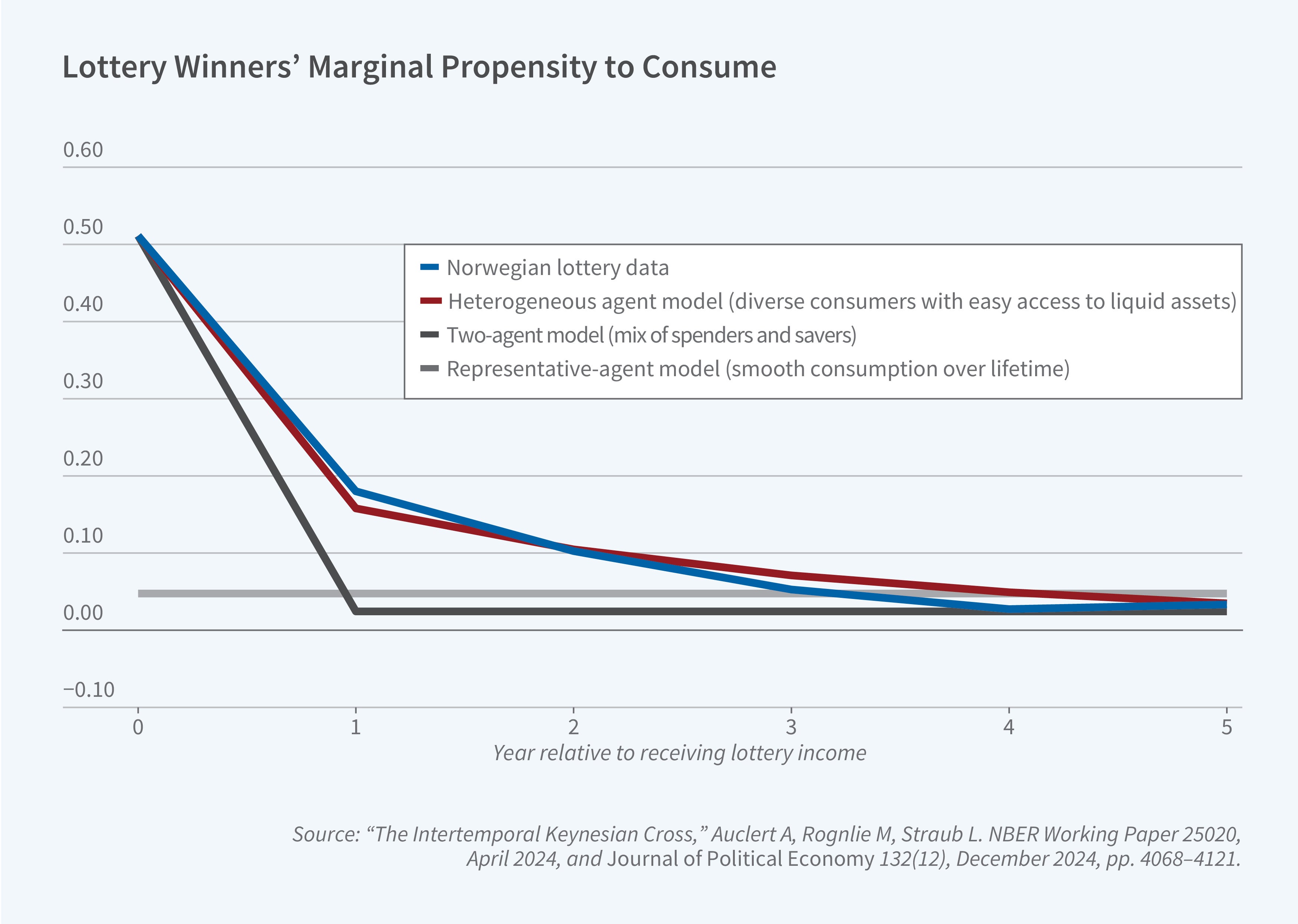
We leverage new evidence on the iMPCs from a Norwegian lottery study that tracks household consumption over several years, visualized in the dots and confidence intervals of Figure 1.² We find that the first-year MPC from receiving lottery income is high, at about 0.5—consistent with many earlier studies—but, importantly, that iMPCs also remain elevated in the second through fourth years after receiving lottery income.

The implication for the effects of fiscal transfers is that these transfers boost aggregate spending not just in the year in which they are sent, but in the next few years as well. Further, higher spending in any year will boost income in that year and therefore spending in earlier and later years. We show that, in simple modern dynamic models, this process can be captured by an “intertemporal Keynesian cross” (IKC). In the IKC, the iMPCs shown in Figure 1, together with the impulse responses of consumption to anticipated future income, turn out to be sufficient statistics for the dynamic effects of fiscal policy on output.

Heterogeneous-Agent Models and the Trickling-Up Process

Because evidence on anticipatory spending effects is relatively scant, and because (outside of the simple case of the IKC) we also need to know the spending response to other shocks such as changes to interest rates, we now look for models that can match the iMPCs from the data. Traditional, representative-agent models are nonstarters because they imply extremely low MPCs, as depicted in the light grey line of Figure 1.

It is common to match high MPCs with saver-spender models, in which a fraction of the population lives hand-to-mouth. These models can explain the high initial MPC in the data (the dark grey line in Figure 1), but not the subsequent high MPCs because the only agents saving their lottery earnings are those with very low MPCs in every period. 

A model with heterogeneous agents facing income risk, borrowing constraints, and a choice between liquid and illiquid accounts matches the iMPC data much better, as shown in the red line of Figure 1. The reason for this success is that consumers in the model accumulate balances after one-off transfers as a way to smooth consumption, but then deplete these balances more quickly than in a representative-agent model as they return to their target balances in each account. Heterogeneity in the speed at which households spend down their wealth is essential to understanding the MPC dynamics in the data. 

In general equilibrium, after deficit-financed transfers of the type that we saw during the recent COVID-19 recession, households who spend down their wealth the fastest—typically poorer, more constrained households—raise the income and wealth of those who do not spend as quickly. This process keeps going, with aggregate spending remaining elevated until the wealth ends up in the illiquid accounts of agents who spend near zero. This “trickling-up” process³ implies that aggregate consumer demand, and therefore inflation, can remain persistently high in the wake of large-scale fiscal transfers. Indeed, elevated inflation and robust consumer spending were observed in many countries for years after their governments sent out COVID-19 relief checks.

Monetary Policy, Micro Jumps, and Macro Humps

In the simplest version of the IKC analysis, monetary policy holds real interest rates constant when fiscal policy changes. What happens when monetary policy raises interest rates instead? 

For the simplest heterogeneous-agent new Keynesian models, it is well understood that the aggregate effect of changes in monetary policy may be quite similar to that in representative-agent models.⁴,⁵

But these models have a flaw with respect to the macro data: they imply an immediate reaction of aggregate consumption and GDP to monetary shocks. This prediction is at odds with most of the macro-empirical evidence on the effects of monetary policy, as well as Friedman’s famous dictum that monetary policy operates with “long and variable lags.” In order for our models to be usable for monetary policy counterfactuals, they need to match both the “micro jumps” (the high iMPCs out of income transfers from Figure 1) and the “macro humps” (the delayed response of aggregate spending to monetary policy).

Our research shows that this can be achieved by assuming that households’ expectations of macroeconomic variables adjust sluggishly following aggregate shocks.⁶ Such departures from rational expectations are widely perceived as difficult to implement for heterogeneous-agent models, but we provide new tools to make computation tractable. The resulting framework is currently serving as a basis for heterogeneous-agent models at several leading central banks around the world. 

With sticky expectations, the response of aggregate consumption to changes in interest rates is very small. In order to explain why monetary policy has any effect at all, we therefore need to rely on the interest-rate responsiveness of other components of aggregate demand. In our model, it is investment that plays this role: by responding to interest rates, investment affects aggregate demand and income, which ultimately drives consumption, thanks to high MPCs. 

Application to Heterogeneous Firms

The sufficient-statistics approach to heterogeneity goes beyond its application to aggregate consumption with heterogeneous households. We can apply it, for instance, to aggregate investment with heterogeneous firms. 

It is well understood that firms have heterogeneous responses to changes in their cash flows, in large part because of heterogeneity in financial constraints: some firms can easily raise additional funds, while other firms must rely on internal financing for all their investment. 

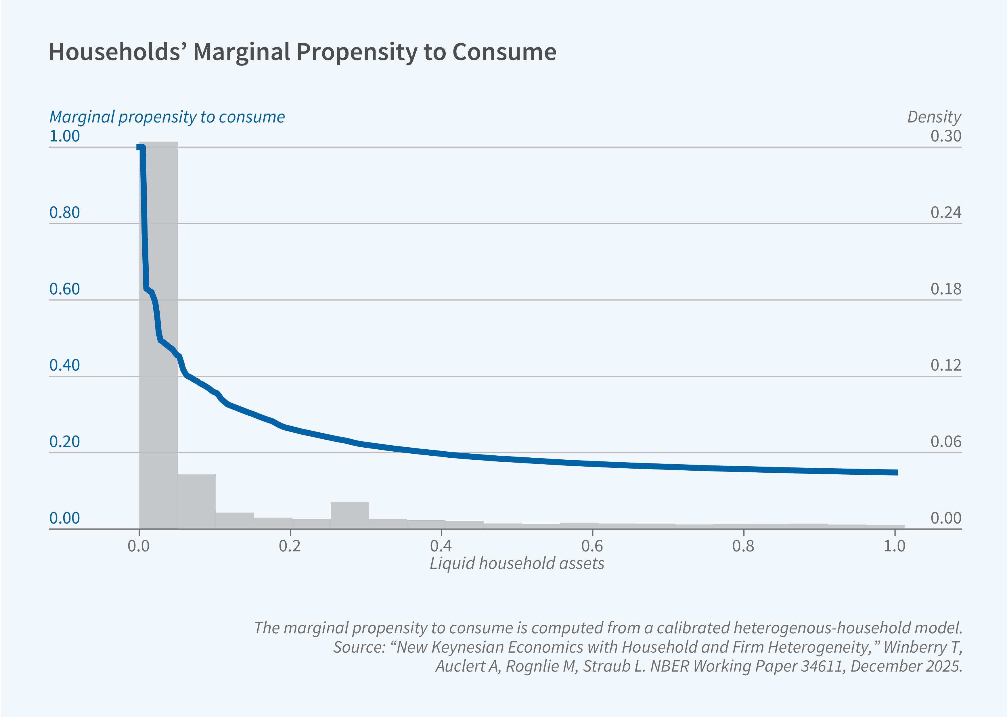
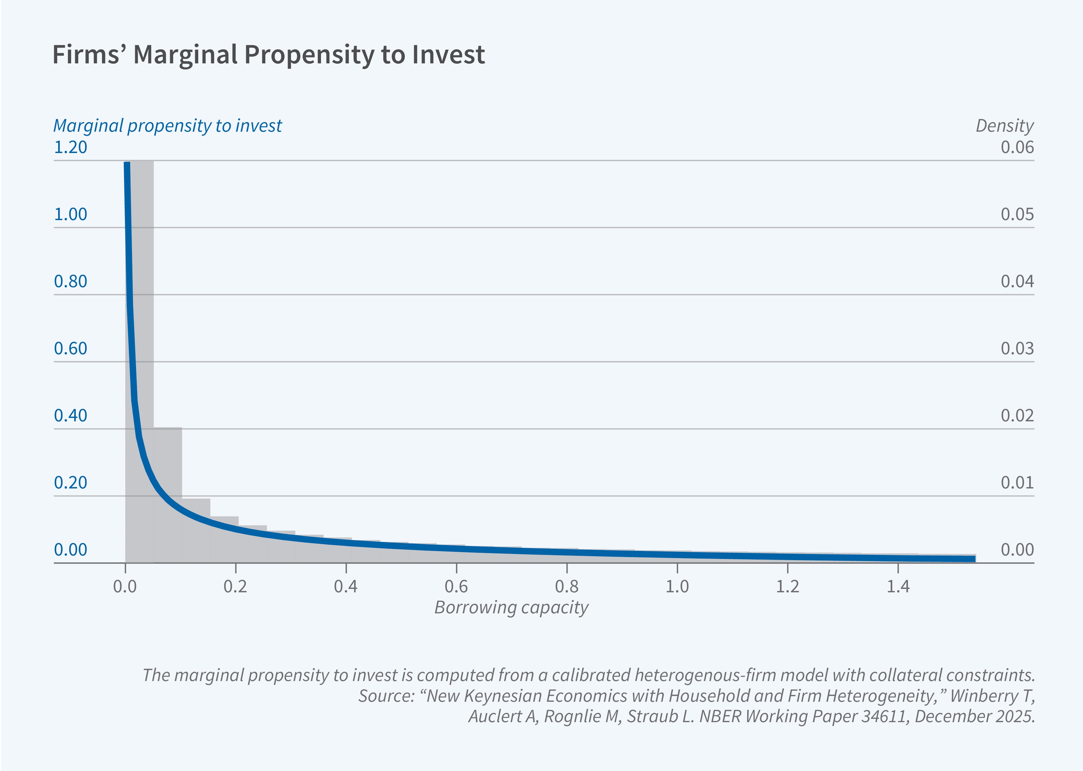
We show that, for the output effects of monetary and fiscal policy, this heterogeneity can be summarized by the distribution of firms’ marginal propensity to invest, or MPI—that is, the response of investment to an unexpected one-time transfer.⁷ In models with heterogeneous firms facing idiosyncratic productivity shocks, entry and exit, and financial frictions, the MPI behaves very similarly to the MPC for households: it is highest for firms near their borrowing constraints (compare the blue curves in Figures 2 and 3). In addition, just as there are many households with low liquid assets, there are many firms with low borrowing capacity (see the distributions in the gray bars of Figures 2 and 3). This implies that both the average MPC and the average MPI can be large in practice. Consequently, transfers to firms can be one way to boost aggregate demand, just like transfers to households.

Sufficient Statistics as a Solution Method

Sufficient statistics are very useful for connecting heterogeneous-agent models to micro data. But we have found that they have another benefit: they make it computationally easier to solve these models in general equilibrium. The traditional “state-space” approach keeps track of the entire distribution of heterogeneous agents in an economy, which can be prohibitively costly once we have rich heterogeneity. But in most models, agents do not directly care about the whole distribution—they care only because of its effects on macro variables such as interest rates and wages. We summarize the macro feedbacks between these variables using “sequence-space Jacobians” and show that these are sufficient statistics for the first-order solution of heterogeneous-agent models, which can be solved very rapidly in practice.⁸

Application to Trends in Long-Run Interest Rates

The sufficient-statistics approach to heterogeneity also goes beyond the analysis of short-run stabilization policy. We can apply it, for instance, to understanding long-run trends in interest rates.

A major hypothesis for the downward trend in real interest rates observed since the 1980s is population aging: as people prepared for long periods of retirement, they demanded an ever-increasing amount of assets. A popular thought is that this trend will reverse as baby boomers age and start to deplete their assets. We show that the effect of population aging on aggregate asset demand and interest rates can be captured by a simple calculation that shows how many assets there will be in the future if we assume that people will accumulate the same amount of assets as they do today relative to earnings, but the age distribution shifts. This calculation is visualized in Figure 4. 

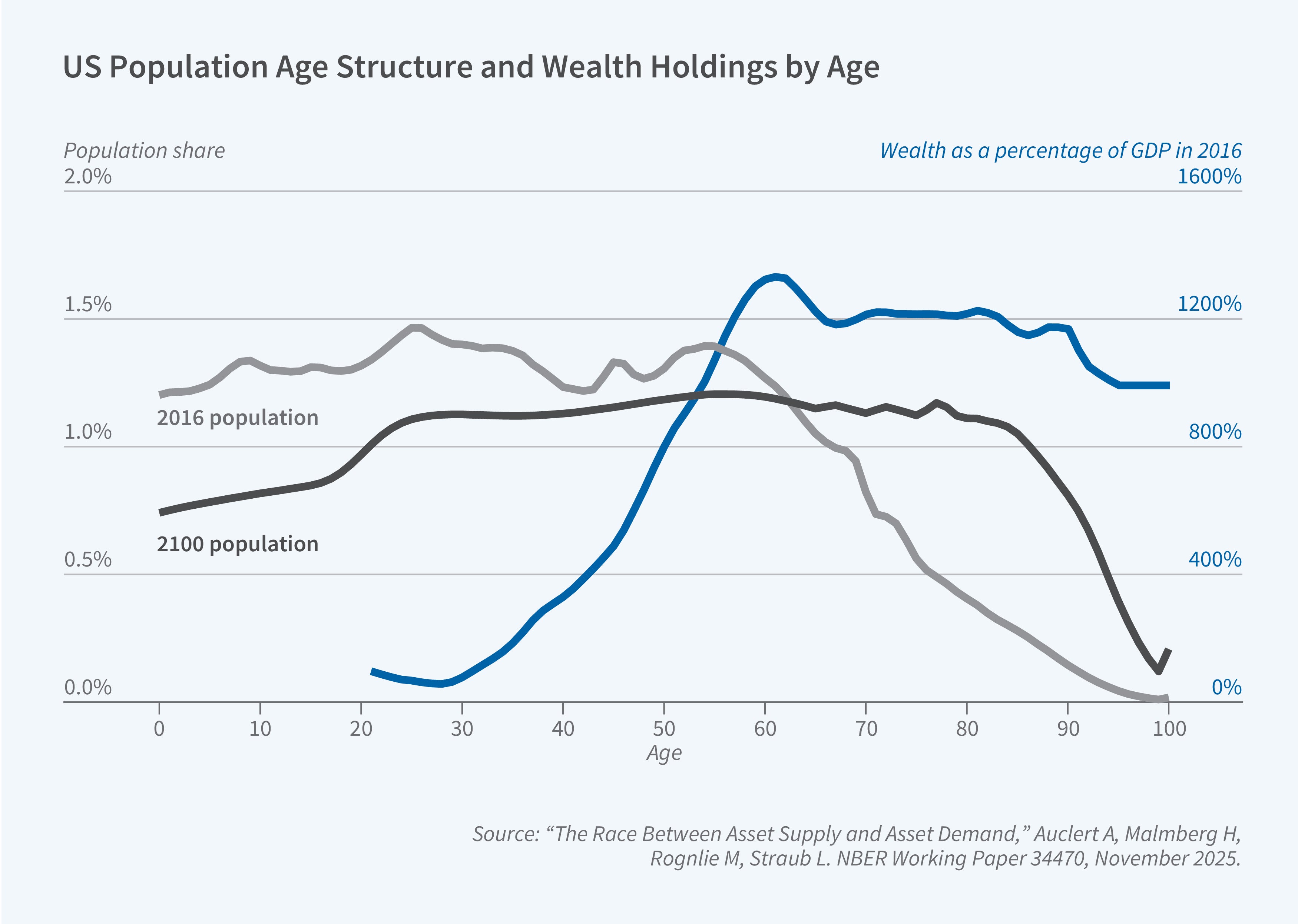
We find that there will be no reversal of this wealth accumulation trend in the decades to come because there is very limited wealth decumulation at old ages. The idea that a decline in asset demand will start pushing up interest rates in the future is therefore not borne out by the data.

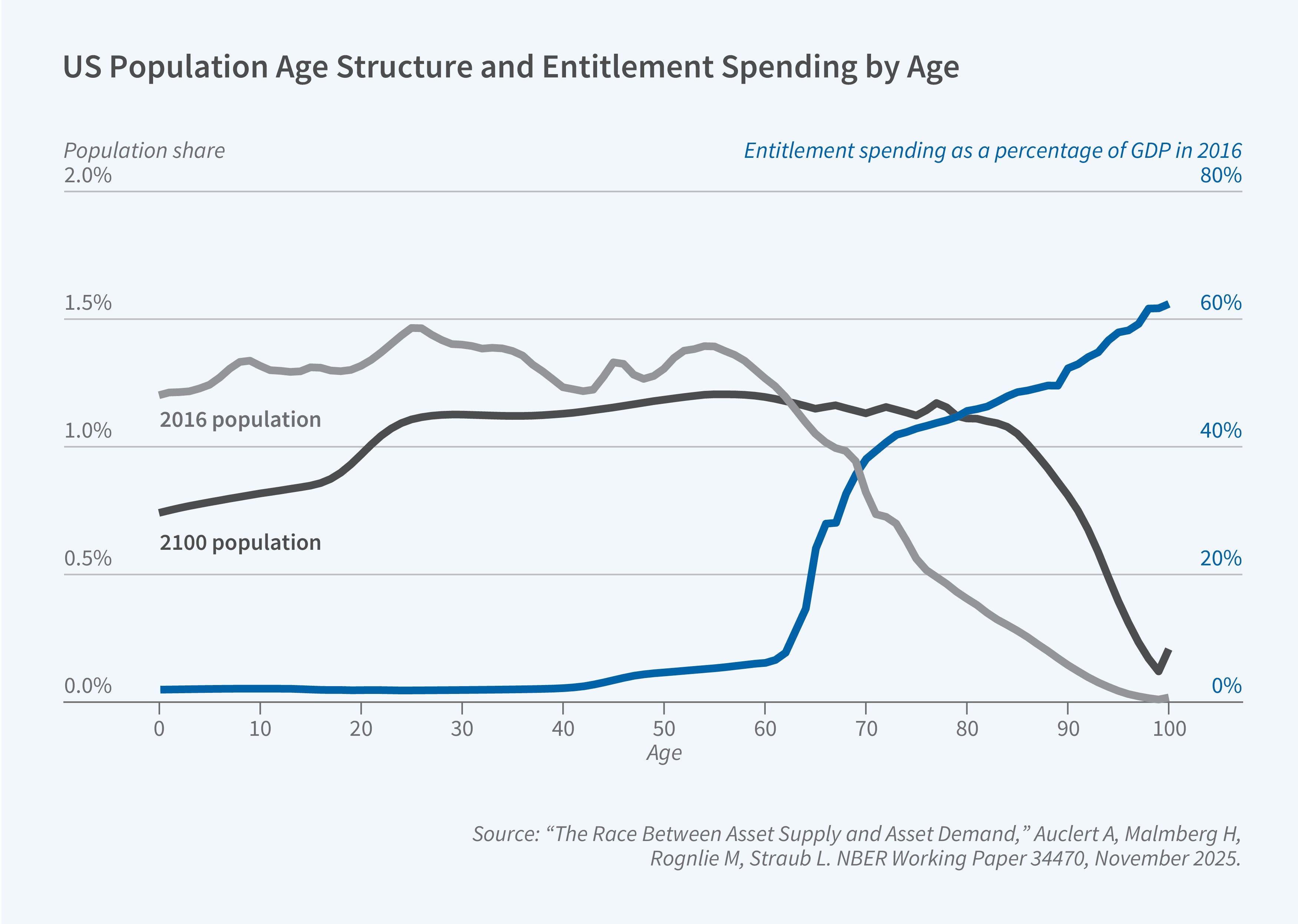
On the other hand, there is another major effect of demographic change: it pushes up aggregate fiscal expenditures because many large programs such as Social Security and Medicare become more generous as people age. Historically, governments have tended not to immediately raise taxes to counteract this effect, leading to deficits that can be forecast with a similar shift-share analysis, visualized in Figure 5. These deficits imply a steady increase in government debt until fiscal adjustment eventually occurs. Until such an adjustment, the supply of assets rises and puts upward pressure on interest rates.

To conclude, demographics may in fact push up interest rates in the decades to come, but if so, this will be despite plentiful savings—as high government deficits outpace individuals’ increasing desire to hold assets.⁹