How Microeconomic Disruptions Affect the Macroeconomy

Aggregation is a central problem for macroeconomics—how to reason about aggregate economic statistics that are composed of many heterogeneous and interacting parts. For example, how do energy shocks, like disruptions to the supply of Russian gas or Middle Eastern oil, affect real output and consumption in Europe and the United States? How do changes in consumer spending behavior during the COVID-19 pandemic affect employment and inflation? How do tariffs on Chinese goods affect real wages in the United States? How does churn in the supply chains of firms—additions and separations of suppliers—affect real output? The common element in these questions is their granularity: The economic shock is not aggregate in nature and affects different parts of the economy differently. The economist’s job is to sum up all the disparate effects, take into account relevant interactions, and produce an estimate of the overall effect on output or consumption. These are not new questions, and in recent decades there has been an explosion of research attempting to answer granular questions like them. In this summary, I describe some key takeaways from this research that tackle a range of applied questions.

The Fundamental Theorem of Aggregation

To begin, consider an idealized perfectly competitive economy. Perfect competition means all producers make decisions taking current prices as given—that is, producers do not alter their behavior to change market prices. Other than this idealization, the economy is arbitrarily complicated. This means the economy may have many different households, each with their own preferences, incomes, and spending patterns. It can also have many producers with complex and interconnected supply chains that span industries and international borders.

How does a small change to one part of this economy affect aggregate output? At first glance, one may imagine that the answer to this question is almost impossibly complex and should depend on all sorts of details. For example, we must know how easy it is to find substitutes for the good being shocked. How complex are the supply chains leading to and the demand chains emanating from this good? How quickly and easily can labor and capital markets reallocate labor and capital? How big are adjustment costs? And on and on.

Surprisingly, the answer turns out to be deceptively simple: the percentage change in output is equal to the sales of the part of the economy that was shocked multiplied by the percentage change in its microeconomic efficiency. So, for example, if oil producers become 1 percent less efficient—that is, they produce 1 percent less output holding their inputs constant—then aggregate output falls by 1 percent times the sales of oil producers relative to total production.

This result, oftentimes known as Hulten’s theorem, is a consequence of perfect competition and underpins my approach to thinking about how granular shocks affect aggregate outcomes.¹ If details other than sales shares matter, then it must be the case that Hulten’s theorem does not apply, and understanding why the theorem fails to apply is key to understanding why its naïve application may over- or understate the true effect. It also highlights what forces are important to measure if we are to arrive at more reliable answers. In each of the research applications below, I discuss the prediction from Hulten’s theorem as well as its shortcomings.

The Effect of Large Disruptions on Output: The Case of Energy

The late Emmanuel Farhi and I extended Hulten’s theorem beyond small shocks.² If the disturbance to the economy is large, then Hulten’s theorem can cease to provide a good approximation. A good example is the energy industry. If the shock is small, then assuming perfect competition, the loss in aggregate efficiency is the reduction in the efficiency of oil producers times their sales as a share of GDP. In normal times, the sales share of energy is small, around 2 percent of GDP. However, a negative shock to oil supply causes oil’s sales relative to GDP to rise.

Figure 1, which plots oil sales relative to GDP, provides an illustration of this phenomenon. In the 1970s, the global economy was buffeted by a series of negative supply shocks to oil, including the Arab oil embargo, coordinated action by members of OPEC, and the Iranian Revolution. Oil sales relative to GDP were 2 percent in 1972 and almost 8 percent in 1980. This means that the same-sized negative shock to the oil industry was four times more damaging to the world economy in 1980 than it would have been in 1972. It also means that, since the sales of oil relative to GDP increased dramatically, Hulten’s approximation would have understated the importance of oil shocks by roughly a factor of three.

The key insight of approaching the problem through the lens of Hulten’s theorem is that it points to an important sufficient statistic for understanding the aggregate consequences of large shocks: changes in sales shares relative to GDP. The forces that cause expenditures on oil to increase relative to GDP in response to negative supply shocks are the same ones we need to understand in order to quantify the effect of those supply shocks on aggregate output. Those forces include complementarities in production technologies between oil and other inputs, diminishing returns to scale that limit the economy’s capacity to maintain energy production in the face of negative shocks, and the ubiquity of oil in supply chains that limits substitution possibilities in the production network.

The Effect of Distortions on Short- and Long-Run Consumption: The Case of Sanctions

In subsequent work, Farhi and I extend Hulten’s theorem to relax the assumption about perfect competition.³ The power of Hulten’s theorem derives from the fact that in a perfectly competitive economy, every potential user and producer of a good has the same valuation for that good. This has two implications. First, since all users of a good have the same valuation for that good, the increase in aggregate output from an increase in the production of a good depends on the sales of that good. Second, reallocations of resources across competing uses are irrelevant; one consumer’s gain is equal in value to another’s loss and has no effect on aggregate output.

When competition is imperfect, due to, say, market power, financial frictions, or taxes, then neither of these statements hold. First, since the costs to producers are not equal to the price faced by consumers, the increase in output from an increase in the production of a good is not approximated by its sales. Second, since the value of a good is not equalized across all market participants, reallocations cannot be ignored, even if one is only interested in aggregate output. Our work develops extensions of Hulten’s theorem to account for these effects in a closed economy without trade.⁴ We also extend this methodology to account for international trade. Hannes Malmberg and I further extend this type of analysis to understand long-run outcomes in models with heterogeneous capital goods and capital accumulation.⁵

We show that, from a long-run perspective, there is a gap between the cost of maintaining the physical capital stock of a country (given by investment costs) and the revenues the capital stock generates (capital income). We show that this gap, which reflects compensation for risk and discounting, is equivalent to a markup on capital services from the perspective of long-run outcomes. For this reason, Hulten’s theorem cannot be naïvely applied to studying long-run outcomes since investment costs are typically not equal to capital income. For example, in the United States, investment is around 20 percent of GDP, whereas capital income is around 35 percent.

In recent work with Malmberg, we apply this methodology to understand how sanctions on Russian energy and a US trade war affect long-run consumption and real wages.⁶ We show that accounting for this gap and modeling capital adjustment is critical when analyzing the long-run effects of trade wars on real wages and consumption. This is because sanctions increase the relative price between investment goods and labor by taxing imported investment goods and their inputs. This price shift depresses capital demand, shrinks the long-run capital stock, and pushes down consumption and real wages compared to scenarios with fixed capital. The extent of the reduction in long-run consumption, in turn, depends on the gap between investment and capital income.

For example, in the case of a US trade war, we show that when adjustments in the capital stock are taken into account, long-run consumption and wage responses are both larger and more negative. With capital adjustment, US consumption can fall by 2.6 percent, compared to 0.6 percent when capital is held fixed.

The Effects of Lumpy Production for Aggregate Productivity: The Case of Supplier Turnover

An assumption implicit in Hulten’s theorem is that production processes can be adjusted smoothly. However, certain production processes cannot just be smoothly scaled up or down. Instead, these changes occur in “lumps”—big jumps in capacity or cost when expanding or shrinking. This is especially true for the entry and exit of firms, which require a minimum size in order to be viable.

Ariel Burstein, Cédric Duprez, Farhi, and I generalize Hulten’s approach to allow for jumps associated with the appearance or disappearance of firms.⁷ Figure 2 shows, at the microeconomic level, the causal impact of the appearance or disappearance of a supplier for the per-unit costs of manufacturing firms in Belgium. The appearance of new suppliers tends to lower costs, and the disappearance of suppliers raises costs for downstream firms. The effect is symmetric and persistent: For each 1 percent of suppliers added or lost, per-unit costs fall or rise by around 0.3 percent as a share of total variable costs. In a perfectly competitive model, where Hulten’s theorem holds, this effect should be zero. If a supplier’s disappearance raises or lowers unit costs for its customers, then it is not rational for that supplier to take prices as given.

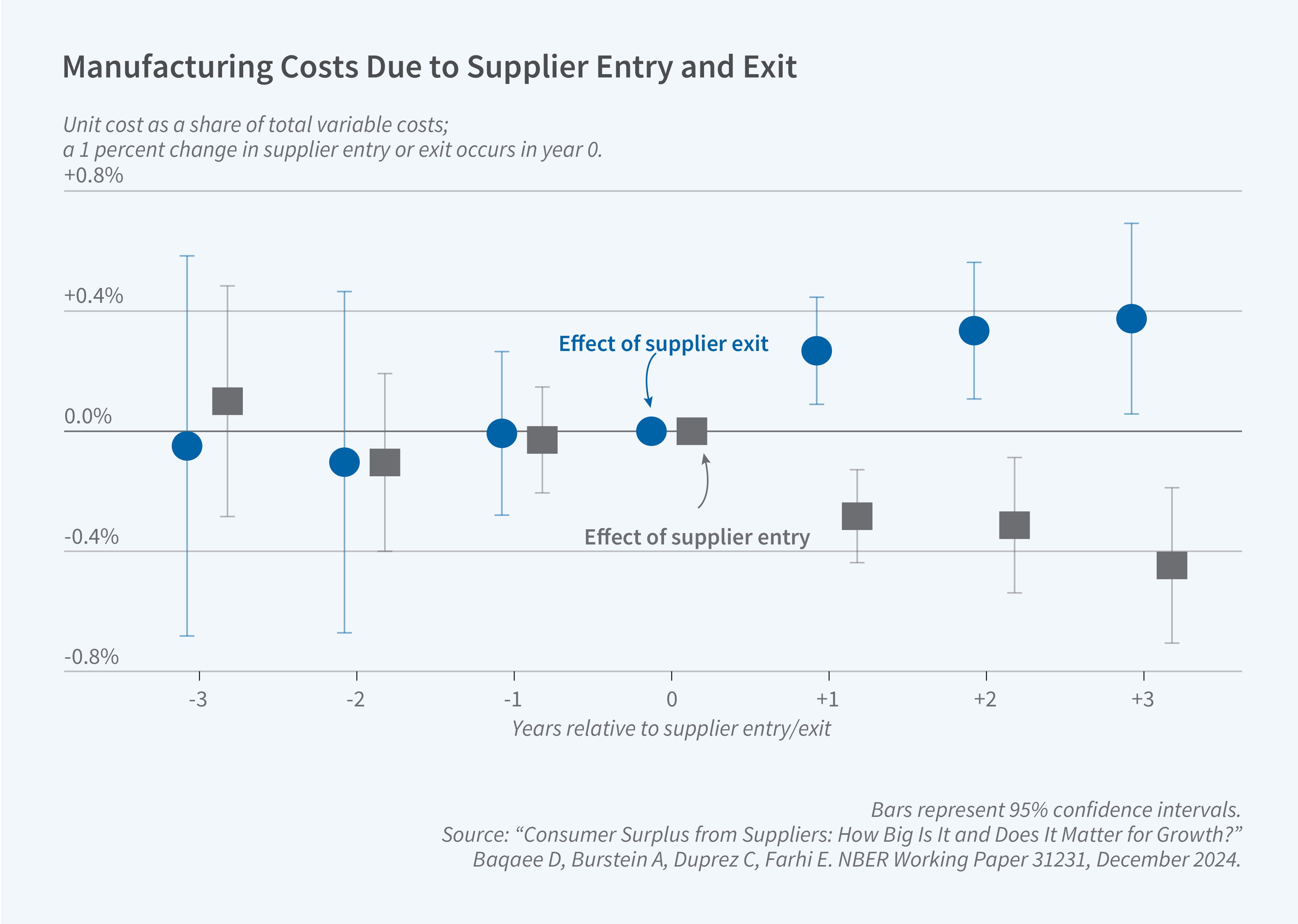
Figure 2 hints at the macroeconomic importance of supplier churn. Dynamism in supply chains, where new suppliers enter into supply chains, pushes down production costs for other firms and boosts aggregate productivity. We quantify the importance of supplier churn for measuring aggregate growth by adding an extensive margin for supplier additions and separations to standard growth accounting formulas based on Hulten’s theorem. Our formula accounts for the effects of supplier link formation and separation on the prices for downstream firms and the transmission of these price changes along existing supply chains from supplying firms to purchasing firms, all the way down to final consumers.

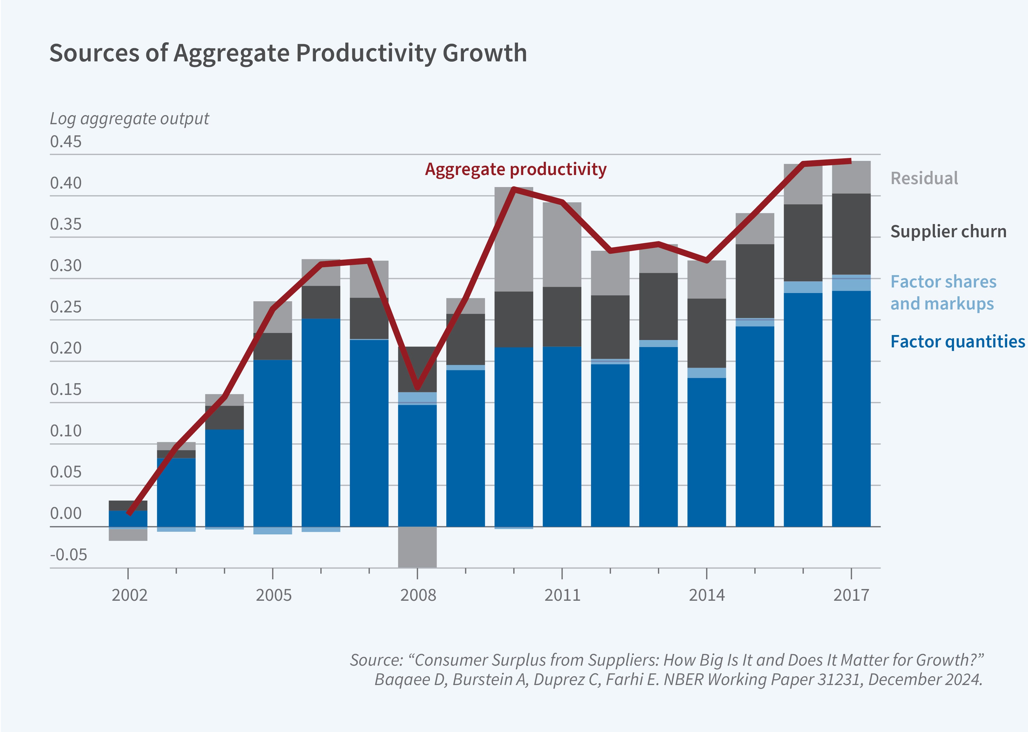
In Figure 3, we use the estimates in Figure 2 plus the Belgian firm-level production network, constructed from value-added tax returns, to conduct a growth accounting exercise for Belgium. We decompose aggregate output growth into several components: growth in the quantity of primary factors like labor and capital, reallocation effects captured by changes in markups and factor shares, a term capturing the importance of supplier churn, and a residual that captures all other factors. We find that around half of aggregate productivity growth—growth not due to factor quantities—between 2002 and 2018 can plausibly be accounted for by supplier churn. This is because each year more suppliers are added than are dropped, in expenditure share terms, and this dynamism in the supply chain can explain a large chunk of aggregate productivity.