The Economic Impact of Climate Change over Time and Space

Climate change is an unintended consequence of the industrialization of the world economy. The evidence that human activity has released large amounts of CO₂ into the atmosphere, leading to rising global temperatures, is by now uncontroversial. However, so far, the scientific and political recognition of this reality has not translated into a commitment to emissions reductions sufficient to stop further global warming. As a result, economists are tasked with evaluating the economic costs of climate change and designing policies to address them. These evaluations are essential: the world cannot embark on ambitious attempts to reduce carbon emissions if we are not reasonably confident that the benefits of these actions will outweigh their costs.

Evaluating the economic impact of climate change is difficult. First, there is the natural science. Models that map carbon emissions to changes in global and local temperatures are readily available, but the mapping of many other physical impacts, such as sea level rise, extreme weather events, or nonlinearities in the climate system, is more complex. While our understanding of these effects is rapidly improving, as shown by the recent Intergovernmental Panel on Climate Change report, there are still no good off-the-shelf models that we can easily plug into our economic analysis.

Second, climate change evolves relatively slowly, unfolding over decades and centuries rather than over months and years. While anthropogenic temperature change is already affecting our present-day reality, many of its more pernicious effects will only be felt in the distant future. Evaluating the implications of warmer temperatures in the far-off future requires dynamic models, as recognized since the pioneering work of William Nordhaus. These protracted effects limit the usefulness of reduced-form empirical studies: extrapolating so far out of sample is undesirable and does not recognize the capacity of humans to react, respond, and adapt to changing circumstances. The Lucas critique — that historical data on the results of economic policy cannot be used to accurately predict the consequences of future policy because people’s behavioral responses also change over time — bites hard here.

Third, CO₂ emissions are a global externality with local economic impact. Because CO₂ mixes rapidly in the atmosphere, emissions from anywhere on the planet lead to changing temperatures across the globe. As a result, any attempt to evaluate the economic impact of climate change needs to be global in nature. At the same time, an aggregate dynamic model of the world economy is not sufficient if it ignores spatial heterogeneity. How can we discuss the impact of coastal flooding without recognizing the difference between Miami and Dallas, or without considering that people can move inland to escape inundation? And how can we evaluate the cost of a 1°C increase in global temperatures without recognizing that this will result in a more than 2°C increase in the most northern latitudes but only a 0.5°C increase in some equatorial regions? Perhaps more importantly, how can we do a comprehensive evaluation if we ignore the fact that higher temperatures are bound to have very different economic effects in the world’s coldest and warmest areas? Recognizing this spatial heterogeneity is essential for an accurate assessment of not just the aggregate impact of climate change, but also the spatial inequality that it might generate.

The Need for Spatial-Dynamic Models

Motivated by these observations, we came to realize the need for economic climate assessment models that take both temporal and spatial dimensions explicitly into account. As temperatures and sea levels change, individuals and firms will respond, and an important part of that adaptation will materialize between, rather than within, locations. Incorporating these behavioral responses requires models with a realistic geography of the world economy that include trade and migration linkages across space. Furthermore, such models also need to recognize that the geography of the world’s productive capacity is not immutable. Where economic activity is concentrated varies significantly over time. The rise of China as a manufacturing powerhouse is but one example of these geographic shifts. As climate changes, areas that benefit from rising temperatures will attract investment and grow. To account for this, climate assessment models should allow growth to endogenously differ across regions.

Over the last decade we have undertaken a research agenda to develop quantitative dynamic spatial models with the goal of evaluating the economic impact of climate change. In doing so, we continue a long tradition of using assessment models that integrate the basic insights of climate science into economic modeling. The difference is that we bring the spatial-dynamic aspect to the forefront. There are various precedents, but we first introduced a model with some of these characteristics in 2014.¹ It features growth and investment in a one-dimensional framework with a continuum of locations, two sectors, costly trade, and free migration.

Temperature Change across Latitudes

In 2015, we used this framework to study the effect of global warming on sectoral specialization, trade, and mobility.² As a first pass, a one-dimensional framework that focuses on differences across latitudes and ignores differences across longitudes is reasonable: a mere 5 percent of the world’s variance in temperature occurs within latitudes.

This research helped us realize the importance of the changing spatial distribution of economic activity in determining the economic cost of global warming. The logic is simple but, we believe, compelling. If moving across locations is cheap, particularly over decades or centuries, and if global warming hurts some places but not others, then changing the spatial distribution of economic activity can be a powerful way to mitigate the losses from climate change. This adaptation mechanism is particularly strong if land is abundant in regions that might benefit from rising temperatures, such as Alaska, northern Canada, and Siberia.

The inevitable conclusion is that the losses from climate change must, to a large extent, be linked to the cost of moving economic activity across locations. These costs are related to moving people and firms. They also depend on trade barriers and on frictions associated with changing local specialization patterns. Additional costs involve leaving behind capital and past investments in local productivity. Losing the agglomeration economies linked to existing clusters of economic activity compounds these costs, even though new population centers sprout up elsewhere.

Modeling the World’s Geography

To more precisely quantify these costs and the spatial frictions faced by agents adapting to climate change, we needed a model with realistic geography. Although a one-dimensional model may be enough to analyze the main effects of rising temperatures across latitudes, it does not suffice to convincingly assess the economic effects of climate change for specific regions in the world and it does not allow use of quantitatively realistic spatial frictions.

In 2018, we developed and quantified a dynamic spatial model with two dimensions, latitude and longitude. Importantly, it features firm investments in local technology that lead to differential local growth in the very protracted transition to a balanced growth path. We used this framework to understand the role of migration and trade frictions in shaping the evolution of the geographic distribution of activity in the world economy.³ Our findings indicate that completely unrestricted migration would increase world welfare by 306 percent. Lending credibility to the framework, a backcasting exercise performed well in predicting population changes across regions over time. More specifically, using a quantification based on data from the year 2000 at a 1° by 1° spatial resolution for the entire globe, we ran the model backward for 50 years and found a correlation between model-implied population changes and actual population changes of 0.74. The fundamental forces in the model can account for many of the changes in the distribution of the world population over half a century without introducing any of the specific local and aggregate shocks that the world economy experienced over this period. Because of these encouraging results, this framework has served as the core economic structure for our subsequent work on climate change.

The Economic Cost of Sea Level Rise

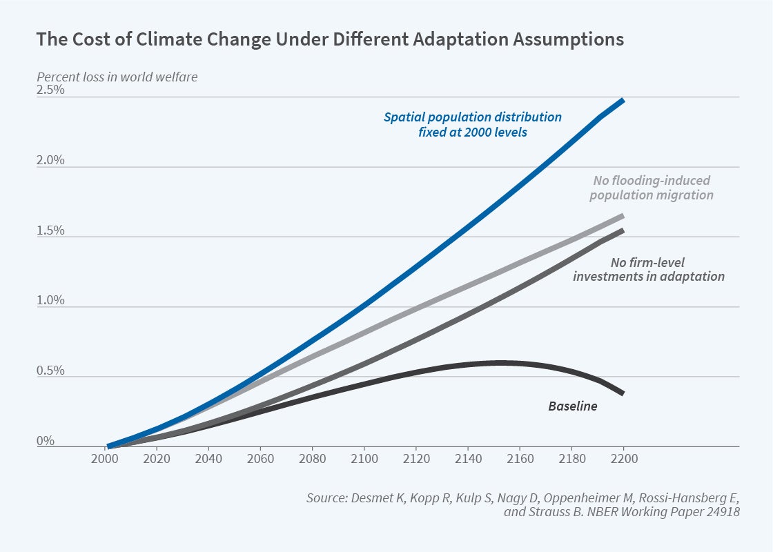
One of the main consequences of a warming world is the global rise in sea levels, expected to surpass half a meter on average by the year 2100. To assess the economic impact of the inundation of coastal areas, we joined forces with climate scientists who generated probabilistic sea level rise projections for various locations around the globe.⁴ Although all oceans are connected, the sea level does not rise uniformly across space, due to differences in factors such as ocean dynamics and tectonics. For example, because of high subsidence, Galveston, Texas is predicted to experience twice the average sea level rise, whereas, because of solid earth responses to regional glacial mass loss, Juneau, Alaska is predicted to experience a drop in its sea level. We combine data on the range of possible paths for the extent of inundation of coastal regions over the next 200 years with our economic model to analyze the economic effect of sea level rise. The result is a probabilistic assessment of the welfare cost of coastal flooding.

Naturally, the ability to move is an effective way to avoid the most harmful impact of rising oceans. Moving is expensive though, and past investments in coastal areas are lost. Still, these costs are substantially lower than when mobility is not considered. Figure 1 depicts the global welfare losses between the years 2000 and 2200 for the median sea level rise projection. Under our baseline estimate (in black), average welfare losses peak around 2150 at roughly 0.5 percent. The figure represents three more scenarios: the static equilibrium (in dark grey) does not allow for changes in firm investments in response to flooding, the fixed population equilibrium (in light grey) does not allow flooding-induced population mobility, and the naïve equilibrium (in blue) keeps the spatial distribution of population as observed in 2000. As expected, when we allow for more forms of adaptation, the negative effect of sea level rise on welfare declines. Going from the naïve scenario with no adaptation at all to our baseline reduces the welfare costs fivefold, from around 2.5 percent to less than 0.5 percent. Of course, sea level rise constitutes only one of the dimensions along which climate change affects the economic environment. It also happens to be a dimension where adapting by moving is particularly useful.

The Geography of Global Warming

In recent work, we have turned our attention from sea level rise to global warming, using a more comprehensive and sophisticated assessment model. We allow changes in local temperatures to influence three local characteristics.⁵ First, changes in temperature affect local productivity, with the impact depending on the location’s initial temperature. Second, changes in temperature have an effect on the attractiveness of a location as a place to live — what is commonly referred to as a location’s amenities. Third, temperature can influence the difference between birth and death rates. Where someone is born matters because migration is costly.

In addition, we incorporate the decision of how much energy to use in production, the choice of the intensity of fossil fuels in generating energy, and the resulting CO₂ emissions of these local choices. Together with a standard carbon cycle model, this yields a framework in which the behavior of the economy affects climate scenarios and vice versa. Incorporating this two-way feedback between local economies and climate is essential if a model is going to be useful in evaluating climate policy.

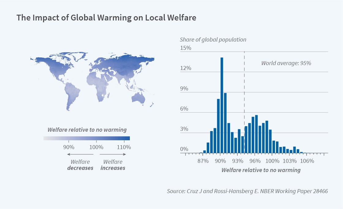
The spatial heterogeneity of the impact of global warming is stark. Figure 2 depicts the cost of global warming across the world’s geography and is expressed as welfare under global warming relative to welfare in a counterfactual scenario where temperatures do not rise. Grey and light blue areas in the map lose, while dark blue areas gain. On average, the world experiences welfare losses of 5 percent, but in the world’s poorest regions losses tend to be substantially larger, as much as 15 percent. The graph in the right panel of Figure 2 presents the population-weighted distribution of these gains and losses. The distribution is bimodal, with many areas of Central Africa, Latin America, and Southeast Asia losing about 10 percent, while many advanced economies lose only marginally and some of the northernmost regions gain. The big story is the spatial heterogeneity of the effects of climate change, and the corresponding augmenting inequality, with the world’s poorest regions being hardest hit.

A core part of the quantification of these welfare losses is the estimation of the damage functions that map changes in temperature to changes in productivity and amenities. Estimating damage functions requires using model-implied fundamental productivities and amenities, rather than final outcomes that already include the many adaptation margins that we are modeling. Using model-implied fundamentals for several periods, we can incorporate local fixed effects and regional trends when estimating the damage functions.

Our damage function estimates suggest that an increase of 1°C in local temperatures implies a decline in amenities of about 2.5 percent in the world’s hottest areas, and a commensurate increase in the world’s coldest areas. The effects of temperature on productivity are larger and asymmetric: a 1°C increase in local temperatures leads to a 15 percent decline in productivity in the warmest regions and a 10 percent increase in the coldest regions. The estimates of these semi-elasticities are statistically significant in the world’s warmest and coldest areas, but the damage functions are estimated with sizable error. This implies uncertainty in the evaluation of global warming. Future research should focus on reducing this error by getting a longer panel of data and by conditioning on not just the mean local temperature, but also on the variance and on the frequency of extreme temperatures.

Trade and Migration as Adaptation Mechanisms

In addition to migration, trade also has the potential to act as a powerful adaptation mechanism. There are, of course, situations where the scope for trade to mitigate the impact of climate change is limited. For example, if global warming affects the productivity of all local firms similarly and if changes in temperature are spatially correlated, trade may not be an effective adaptation mechanism. However, the effect of temperature on productivity likely varies by sector, so trade can help hard-hit locations switch to sectors that are less affected by climate change.

In recent research, we incorporate an agricultural and a nonagricultural sector and evaluate how changes in local specialization may operate as an adaptation mechanism.⁶ Our analysis shows that the role of trade is complex. On the one hand, freer trade increases the scope of local specialization, leading to smaller losses from global warming. On the other hand, freer trade weakens the incentives for people to migrate away from today’s poorest regions, which are more affected by climate change. On balance, we find that freer trade increases losses from global warming in the near future but reduces losses in the far-off future.

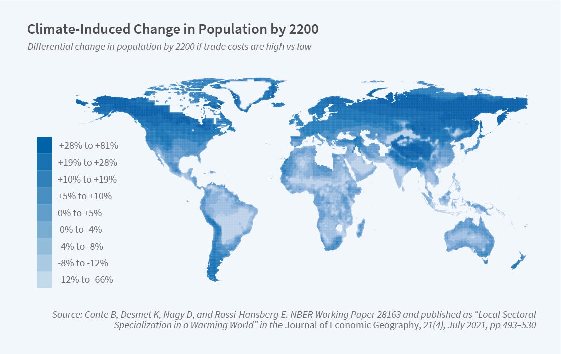
As adaptation mechanisms, trade and migration are substitutes. Figure 3 depicts the climate-induced change in population in 2200 when trade costs are high compared to when trade costs are low. Areas marked in dark blue gain more population due to rising temperatures when trade costs are high, and areas marked in light blue and grey lose more population. The map shows that more people move away from highly affected areas in equatorial regions when trade costs are higher. That is, when trade has less scope to act as an adaptation mechanism, migration plays a bigger role.

What’s Next?

We are continuing to improve our climate assessment model, estimating richer damage functions that incorporate episodic effects and their variance, incorporating anticipatory effects on investments, and adding a richer sectoral composition with input-output linkages. Our agenda includes a thorough evaluation of various environmental policies, including their spatial characteristics and implications.