Program Report: Industrial Organization
Researchers in the Industrial Organization (IO) program study consumer and firm behavior, competition, innovation, and government regulation. This report begins with a brief summary of general developments in the last four decades in the range and focus of program members’ research, then discusses specific examples of recent work.
When the program was launched in the early 1990s, two developments had profoundly shaped IO research. One was the development of game-theoretic models of strategic behavior by firms with market power, summarized in Jean Tirole’s classic textbook.1 The initial wave of research in this vein was focused on applying new insights from economic theory; empirical applications came later. Then came the development of econometric methods to estimate demand and supply parameters in imperfectly competitive markets. Founding program members including Tim Bresnahan, Ariel Pakes, and Rob Porter played a key role in advancing this work.2
Underlying both approaches was the idea that individual industries are sufficiently distinct and industry details sufficiently important that researchers need to focus on specific markets and industries in order to test particular hypotheses about consumer or firm behavior, or to estimate models that could be used for counterfactual analysis, such as analysis of a merger or regulatory change.
There were, to be sure, some points of overlap with neighboring fields. A notable example was the role that industrial organization economists played in the activities of the NBER’s Productivity, Innovation, and Entrepreneurship program, where the research agenda embraced the estimation of plant-level costs and productivity and the effects of firm and market characteristics on R&D spending and the rate of innovation.
The last two decades have witnessed two broad trends in expanding the scope of program members’ research. One concerns topics: while studies of traditional IO questions around antitrust and competition policy have continued to be a key defining area of inquiry for the field, there has been rapid growth of research by NBER IO scholars on sectors such as healthcare,3 education,4 financial markets,5 media,6 and transportation.7 This type of topical expansion is now colloquially termed “IO+.”
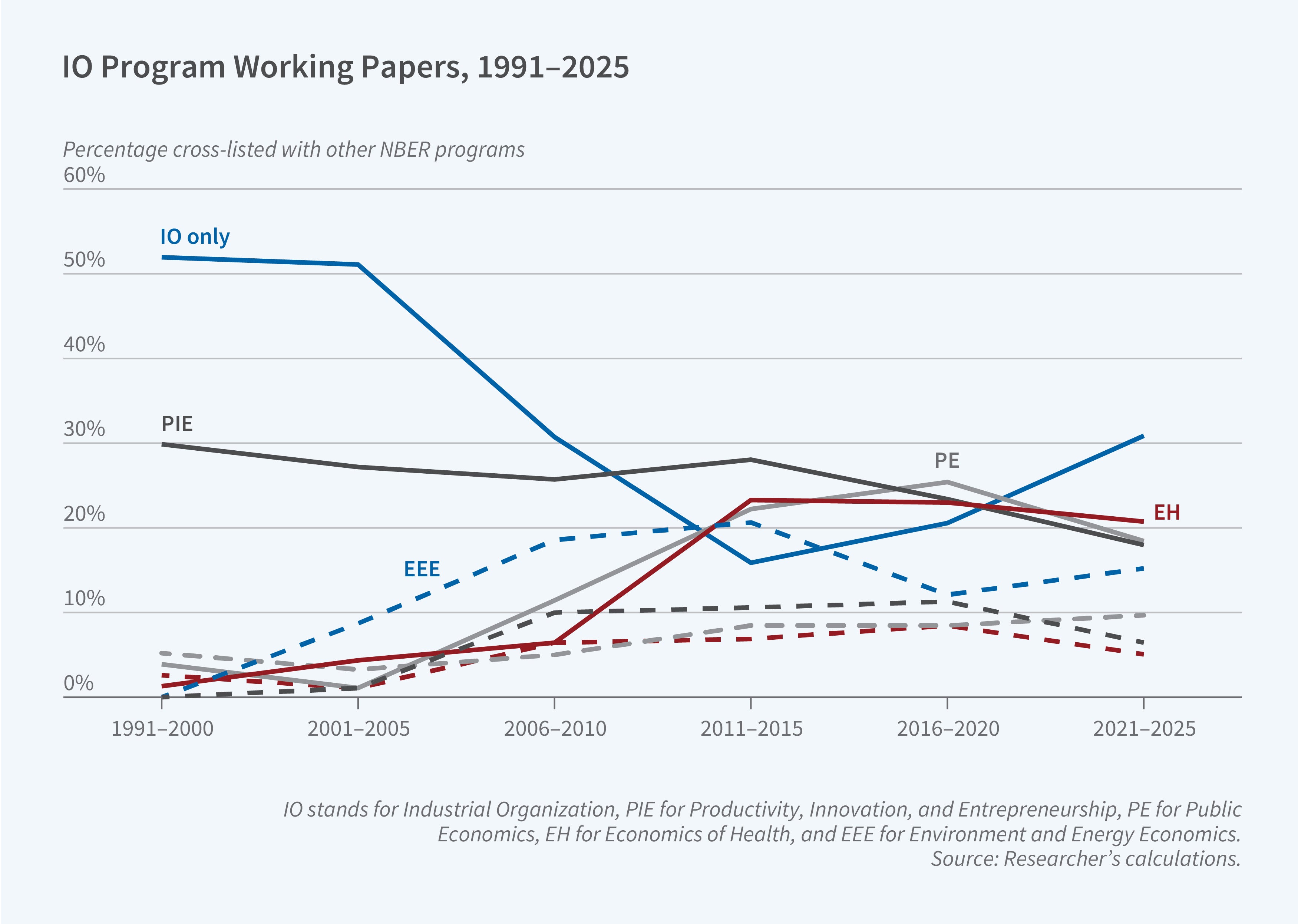
The second trend is more methodological. The empirical work in the 1990s relied heavily on insights from game theory and naturally emphasized structural modeling of demand and supply. This ran somewhat counter to the trend in other applied microeconomic fields at the time, which highlighted natural experiments and causal inference. In the last two decades, we have seen some convergence between empirical IO and other fields of applied microeconomics. Work in other fields is increasingly using “IO-style” econometric modeling, while IO papers increasingly combine (within and across papers) causal inference methods that motivate and complement the subsequent theory-based econometric models.
To illustrate the broadening research activity of industrial organization economists, this summary highlights several specific papers. They have been chosen to underscore the wide spectrum of industries and topics addressed by program members and the variety of approaches and tools being used to study competition and markets. The last section summarizes some more recent IO work on the very active, core IO topics of antitrust and competition policy.
These examples are not meant to be a summary of the much broader scope of research by program affiliates. All of the recent working papers by program affiliates may be found on the NBER website's IO program page.
The Digital Economy
Over the last two decades, the digital economy has grown enormously and today it plays a central role in economies around the world. While some segments of the digital economy are highly competitive, there are growing concerns that incumbent firms have established entrenched positions and wield substantial market power. This has led to ongoing antitrust policy action such as the adoption of the Digital Markets Act in Europe and the legal discourse between Google and the US Department of Justice.
The growing size of and policy interest in the digital economy has been a fertile ground for new research. One recent example, which also illustrates the broad set of empirical tools deployed by IO scholars, is the work by Hunt Allcott, Juan Camilo Castillo, Matt Gentzkow, Leon Musolff, and Tobias Salz8 which studies the dominance of Google in the internet search engine market.
Google has maintained a very stable market share of 80–90 percent, both in the US and worldwide, over the last two decades, and the paper attempts to uncover the determinants of this market dominance. One hypothesis is that Google attracts more users because it is simply better. An alternative is that Google enjoys an advantage due to its status as a default and/or first mover, which in this context may manifest itself by users finding it difficult to switch search engines and/or by users incorrectly perceiving Google to be better because they have had no experience with alternatives (mostly Bing in the US). This question is one of the most foundational in IO: if it is the former then Google’s dominance may be an efficient market outcome, while if it is the latter, there might be a case for policy intervention.
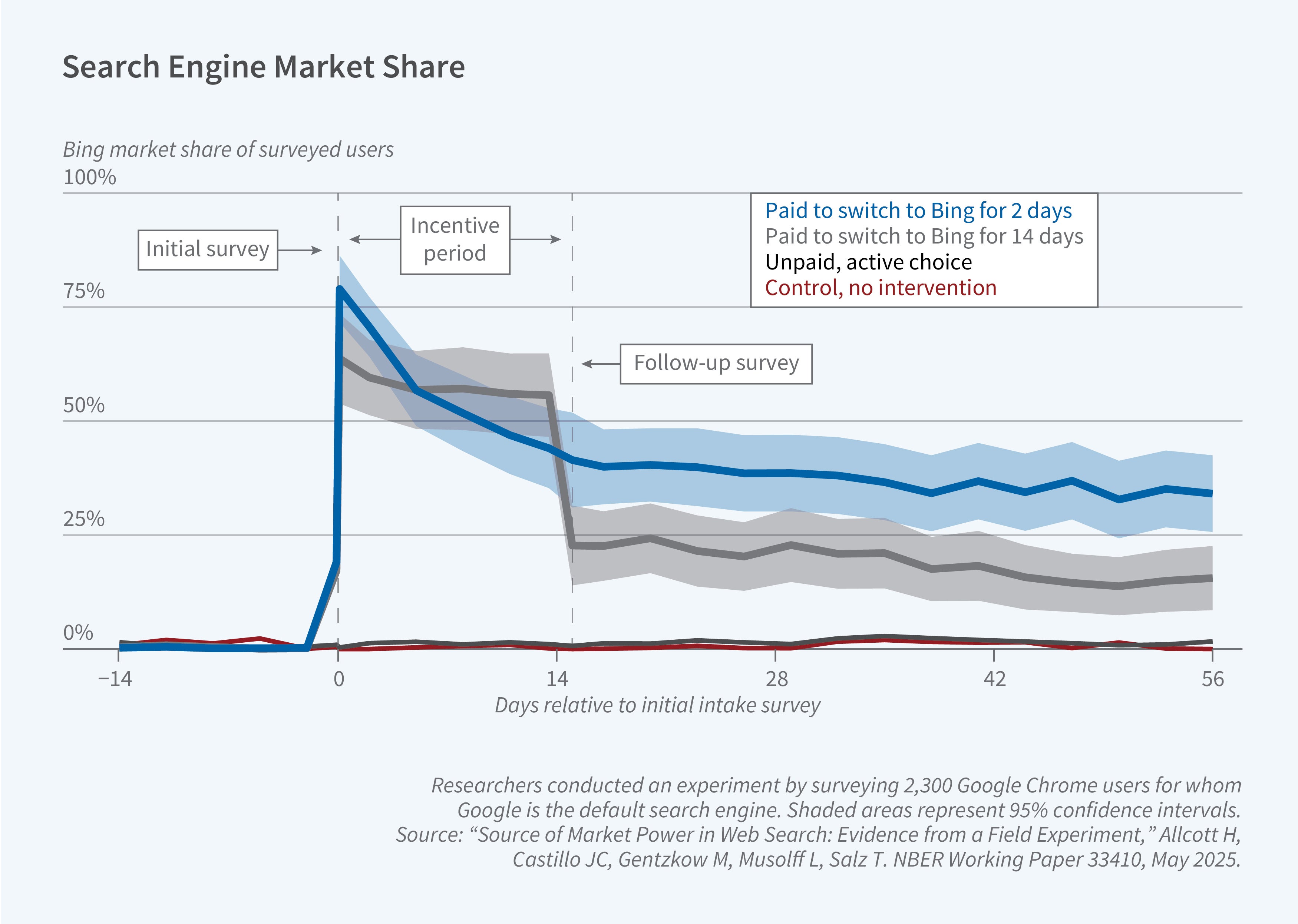
To study this question, the researchers ran a randomized experiment and embedded the experimental results in a stylized model of search engine choice to quantify its implications. They recruited approximately 2,300 Google Chrome users, surveyed them at enrollment (day 0) and two weeks later (day 14), tracked their search behavior, and randomized them into several experimental arms. In one arm, users were forced to make an active search engine choice. A second arm incentivized users to switch to Bing for 14 days, after which they would make an active search engine choice. A third arm incentivized users to change the default search engine. The researchers also cross-randomized an arm that used a browser extension to degrade the quality of users’ search results on Google.
The experimental results are depicted in Figure 2. Forcing users to make an active choice does not have much of an impact, but many users who were incentivized to switch to Bing for 14 days continued to use Bing even after the 14-day incentivized period had elapsed. The 14-day survey also suggests that, on average, those who used Bing had a more positive view of Bing’s quality relative to their day-0 perception.
Embedding these experimental results in a model of search engine choice, the researchers conclude that defaults have a first-order importance in this setting. They estimate that about a third of users are “permanently inattentive,” and this prevents them from learning about other search engines. This helps Google retain its market share because users underestimate the quality of competitors.
The researchers use the results to assess possible remedies to Google’s high market share. They conclude that active choice screens (as implemented in Europe) do not have much of an impact, but changing defaults could significantly reduce Google’s market share. This would benefit some consumers who learn they prefer the alternative, but also hurt many others who prefer Google but would not switch back (once the default changed) due to inattention.
Related work by Michael Ostrovsky9 studies the auction design for spots on the active choice screens in Europe and shows that the auction to get on the active choice menu would be much more competitive if bids were made on a per-install basis rather than on a per-appearance basis, because the latter places small search engines at a major disadvantage.
Another recent and policy-relevant topic of interest in the digital economy context is the question of “self-preferencing” by digital platforms, as many platforms operate as both a platform and as a seller on the platform. This has led to concerns, for example, about potential Google preferences for its own Google Shopping service when displaying search results, or for Amazon self-preferencing Amazon-owned products in its e-commerce marketplace. Papers by Chiara Farronato, Andrey Fradkin, and Alex MacKay10 and by Joel Waldfogel11 present evidence that support this concern by showing that Amazon ranks its own products higher than competitors’ comparable products. The latter paper also shows that the European Digital Market Act has decreased, but has not eliminated entirely, this self-preferential treatment.
Transportation Markets
As mentioned above, the last two decades have witnessed the growth of “IO+” work, which recognizes that the current style of empirical IO work has proven useful in studying a range of markets. Within this overall trend, with the availability of new sources of granular data and the emergence of ride-hailing platforms, transportation markets have gained significant attention from IO scholars in recent years.
One example is a paper by Milena Almagro, Felipe Barbieri, Castillo, Nathaniel Hickok, and Salz,12 which uses data from the city of Chicago to study urban transportation policy. The paper is motivated by the simple fact that the vast majority of Americans commute by car, leading to both congestion and environmental costs. At the same time, the average bus in Chicago, and presumably in many other cities, is well below capacity. The paper explores the extent to which congestion pricing and/or subsidies and improvements to public transit can be effective.
To study this question, the authors assemble a rich dataset from multiple sources for a single calendar month (January 2020) in Chicago: trip-level public transport (trains and buses) data, trip-level data on the universe of taxi and ride-hailing (Uber and Lyft) trips, and private-car trips based on mobile-phone geolocation data (covering about 40 percent of all devices).
The richness of the data allows the authors to estimate a heterogeneous demand system for modes of transportation,13 which sheds light on how individuals trade off convenience, money, and time. The model can be used to evaluate possible changes in public transit pricing and frequency, and in private transit congestion fees. The results suggest that there are welfare gains from free public transit as well as from road pricing and congestion fees. The findings emphasize the interaction between these two potential interventions, highlighting the strong complementarities that emerge from municipal budget constraints.
There are many other recent examples of related work. One is a study by Panle Jia Barwick, Shanjun Li, Andrew Waxman, Jing Wu, and Tianli Xia,14 which uses granular commuting data from Beijing to estimate an equilibrium sorting model and assess various urban transportation policies. A second is the work by Nick Buchholz, Laura Doval, Jakub Kastl, Filip Matějka, and Salz,15 which uses ride-level price variation from a European ride-hailing platform in which cabs bid for rides in order to back out individuals’ value of time. A third example is the work by Giulia Brancaccio, Myrto Kalouptsidi, and Theodore Papageorgiou,16 which uses granular, geolocation trip-level data on marine shipping to develop and estimate an equilibrium model of worldwide international trade.
Market Power and Competition Policy
In addition to some of these newer trends, the last decade has also witnessed renewed interest in some of the core IO questions around measuring markups and market power and assessing the anticompetitive impact of mergers and acquisitions.
One line of work has been driven by the influential paper of Jan De Loecker, Jan Eeckhout, and Gabriel Unger,17 which analyzes Compustat data and applies a macro-style, “production function” empirical approach, that finds that average markups in the US economy have been rising over the last four decades. This striking finding has generated a number of follow-on studies. For example, Ali Yurukoglu, Paul Grieco, and Charlie Murry18 recovered markups in the US auto industry using the more standard IO approach, which relies on inverting the first order condition for optimal pricing. They found that markups in the US auto industry have been, in fact, declining. In contrast, two related papers19 apply a similar “standard IO” approach to consumer-packaged goods and find that markups have increased due to a combination of lower marginal costs and a decline in consumers’ price sensitivity. In a review of recent evidence on the topic,20 Yurukoglu and Carl Shapiro write that “the economic evidence that looks across many industries over a long period of time does not support the view that there has been a widespread decline in competition in the US economy over the past 25 or 40 years.” This remains a subject of lively debate.
The claim that markups are rising has led some to argue that US antitrust policy is too lax. This sentiment, along with recent research on horizontal mergers, contributed to the 2023 revision of the merger guidelines.21One example of recent research is Tom Wollmann’s study22 of “stealth consolidation,” which shows how firms break down one large merger into a sequence of smaller mergers, all of which fall below the reporting threshold and thereby avoid antitrust scrutiny. Another example is the work of Volker Nocke and Michael Whinston,23 who develop several quantitative theory exercises that suggest that consumer welfare can be approximated reasonably well by the magnitude of the change in concentration measure regardless of its initial level. A third recent example of research on related issues is a study by Mert Demirer and Omer Karaduman.24 Using data on thousands of power plant acquisitions in the US, they estimate a 2–5 percent increase in productivity for the average acquisition, providing new evidence about the productivity-enhancing benefits of industry consolidation.
Looking Ahead
This is an exciting time to be carrying out research in industrial organization. The “data revolution” has created many incredible opportunities, including the use of administrative datasets, scalable web scraping, and many collaborations with private companies. The active public discourse around competition policy and “big tech” is a fertile ground for new and impactful work, and the increasing “IO+” research makes it possible for IO scholars to overlap and interact even more than in the past with work and scholars from other fields. NBER IO meetings always cover a vast set of topics and industries and a range of empirical methods, creating many learning opportunities for all of us.
Endnotes
The Theory of Industrial Organization,” Tirole J. Cambridge, Massachusetts: The MIT Press, 1988.
“Entry and Competition in Concentrated Markets,” Bresnahan TF, Reiss PC. Journal of Political Economy 99(5), 1991, pp. 977–1009.
Automobile Prices in Market Equilibrium, Berry S, Levinsohn J, Pakes A. NBER Working Paper 4264, January 1993, and Econometrica 63(4), July 1995, pp. 841–90.
The Role of Information in US Offshore Oil and Gas Lease Auctions, Porter R. NBER Working Paper 4185, October 1992, and Econometrica 63(1), January 1995, pp. 1–27.
Equilibria in Health Exchanges: Adverse Selection vs. Reclassification Risk, Handel B, Hendel I, Whinston M. NBER Working Paper 19399, September 2013, and Econometrica 83(4), July 2015, pp. 1261–1313.
Insurer Competition in Health Care Markets, Ho K, Lee R. NBER Working Paper 19401, November 2016, and Econometrica 85(2), March 2017, pp. 379–417.
Demand Analysis using Strategic Reports: An application to a school choice mechanism, Agarwal N, Somaini P. NBER Working Paper 20775, October 2017, and Econometrica 86(2), March 2018, pp. 391–444.
Heterogenous Beliefs and School Choice Mechanisms, Kapor A, Neilson C, Zimmerman S. NBER Working Paper 25096, December 2019, and American Economic Review 110(5), May 2020, pp. 1274–1315.
The High-Frequency Trading Arms Race: Frequent Batch Auctions as a Market Design Response, Budish E, Cramton P, Shim J. Presented in the NBER IO Summer 2014 meeting, and Quarterly Journal of Economics 130(4), November 2015, pp. 1547–1621.
Bid Shading and Bidder Surplus in the US Treasury Auction System, Hortacsu A, Kastl J, Zhang A. NBER Working Paper 24024, November 2017, and American Economic Review 108(1), January 2018, pp. 147–169.
What Drives Media Slant? Evidence from US Daily Newspapers, Gentzkow M, Shapiro J. NBER Working Paper 12707, August 2007, and Econometrica 78(1), January 2010, pp. 35–71.
The Welfare Effects of Vertical Integration in Multichannel Television Markets, Crawford G, Lee R, Whinston M, Yurukoglu A. NBER Working Paper 21832, April 2017, and Econometrica 86(3), May 2018, pp. 891–954.
Figure 1 presents an attempt to quantify this topical evolution of the field by updating an earlier figure from our 2017 program report.
Sources of Market Power in Web Search: Evidence from a Field Experiment, Allcott H, Castillo JC, Gentzkow M, Musolff L, Salz T. NBER Working Paper 33410, May 2025.
Choice Screen Auctions, Ostrovsky M. NBER Working Paper 28091, November 2020, and American Economic Review 113(9), September 2023, pp. 2486–2505.
Self–Preferencing at Amazon: Evidence from Search Ranking, Farronato C, Fradkin A, MacKay A. NBER Working Paper 30894, January 2023, and AEA Papers and Proceedings 113, May 2023, pp. 239–243.
Amazon Self–Preferencing in the Shadow of the Digital Market Act, Waldfogel J. NBER Working Paper 32299, April 2024.
Optimal Urban Transportation Policy: Evidence from Chicago, Almagro M, Barbieri F, Castillo JC, Hickok N, Salz T. NBER Working Paper 32185, October 2025.
It is impossible to not think about the data revolution in this context. One of the more famous empirical applications that motivated Daniel McFadden’s Nobel-Prize econometric contributions explored a very similar type of question, but had to rely on a survey of 213 Bay Area commuters. (“The Measurement of Urban Travel Demand,” McFadden D. Journal of Public Economics, 3(4), November 1974, pp. 303–328).
Efficiency and Equity Impacts of Urban Transportation Policies with Equilibrium Sorting, Barwick P, Li S, Waxman A, Wu J, Xia T. NBER Working Paper 29012, February 2022, and American Economic Review 114(10), October 2024, pp. 3161–3205.
Personalized Pricing and the Value of Time: Evidence from Auctioned Cab Rides, Buchholz N, Doval L, Kastl J, Matějka F, Salz T. NBER Working Paper 27087, March 2024, and Econometrica 93(3), June 2025, 929–958.
Geography, Search Frictions, and Endogenous Trade Costs, Brancaccio G, Kalouptsidi M, Papageorgiou T. NBER Working Paper 23581, October 2018, and Econometrica 88(2), March 2020, 657–691.
The Rise of Market Power and the Macroeconomic Implications, De Loecker J, Eeckhout J. NBER Working Paper 23687, August 2017. Published with Unger G in The Quarterly Journal of Economics 135(2), January 2020, pp. 561–644.
The Evolution of Market Power in the US Auto Industry, Grieco P, Murry C, Yurukoglu A. NBER Working Paper 29013, July 2021, and The Quarterly Journal of Economics 139(2), May 2024, pp. 1201–1253.
Scalable Demand and Markups, Atalay E, Frost E, Sorensen A, Sullivan C, Zhu W. NBER Working Paper 31230, May 2023, and forthcoming in the Journal of Political Economy.
Rising Markups and the Role of Consumer Preferences, Döpper H, MacKay A, Miller N, Stiebale J. NBER Working Paper 32739, July 2024, and Journal of Political Economy 133(8), August 2025, pp. 2462–2505.
Trends in Competition in the United States: What Does the Evidence Show? Shapiro C, Yurukoglu A. NBER Working Paper 32762, August 2024, and forthcoming in the Journal of Political Economy Microeconomics.
The revised guidelines have benefited from important contributions by NBER IO members, Susan Athey and Aviv Nevo who served at the time as chief economists of the Department of Justice and Federal Trade Commission, respectively.
How to Get Away with Merger: Stealth Consolidation and Its Effects on US Healthcare, Wollmann T. NBER Working Paper 27274, March 2024.
Concentration Screens for Horizontal Mergers, Nocke V, Whinston M. NBER Working Paper 27533, July 2020, and American Economic Review 112(6), June 2022, pp. 1915–1948.
Do Mergers and Acquisitions Improve Efficiency? Evidence from Power Plants, Demirer M, Karaduman O. NBER Working Paper 32727, July 2024, and forthcoming in the Journal of Political Economy.