Beliefs, Tail Risk, and Secular Stagnation

Beliefs govern every choice we make. Much of the time, they lie in the background of our economic models. We often assume that everyone knows everything that has happened in the past, as well as the true probabilities of all future events. The concept of rational expectations means that the true distribution of future outcomes and the believed distribution of future outcomes are the same.

     If the rational expectations assumption were true, there would be no need for economists. If everyone knew all covariances, we would not need any empirical work. If everyone knew the true model of the economy and could reason through it, we would not need theorists. Luckily for us, the rational expectations assumption is not correct.

    Yet most of the time it is a useful simplification. We have seen enough economic booms and recessions, firm and bank failures to have a reasonable estimate of their true probability. However, when studying rare events, often referred to as “tail events,” assuming rational expectations can lead economists astray. Because these events are rare, data on them are scarce, and our estimates of their true probability are unlikely to be accurate. In these circumstances, understanding belief formation becomes particularly important.

    My research focuses on how individuals, investors, and firms get their information, how that information affects the decisions they make, and how those decisions affect the macroeconomy and asset prices. It also examines how people form beliefs about tail risk and how learning about tails, or disasters, can explain persistent low interest rates, volatile equity prices, and secular stagnation.

Belief Formation

    There are two broad approaches to explaining belief formation. The first is a behavioral approach, which departs from rational expectations by directly stating some belief formation rule that explains the phenomenon at hand. Such assumptions are often supported with survey or experimental data. These assumptions may be right, but they rarely provide a reason for the agents' beliefs. If we don't understand why the rule holds, we don't know in what circumstances the rule will continue to hold. While such approaches provide insights, there is more to be discovered.

    The second approach to belief formation is an imperfect-information approach. Agents have finite data to estimate states and distributions. Despite the limited information, they estimate efficiently, given the data they have, or the information they have optimally chosen to acquire, attend to, or process. Agents in these models do what economists would do if we were in their place: They collect data and use standard econometrics to estimate features of their environment. When a new outcome is observed, they re-estimate their model in real time.

    The imperfect-information approach overcomes one of the main challenges of working on beliefs — the fact that beliefs are hard to observe or measure. Survey data are informative in many circumstances, but reporting accurate probabilities of rare events is particularly difficult, and surveys are rarely designed to elicit these beliefs. Also, when beliefs change on short notice, capturing this change with surveys is usually infeasible because of the costly and time-consuming nature of survey administration. In contrast, when we model agents as econometricians, we can estimate their beliefs in real time with publicly observable data and standard econometrics.

Tail Risks, Secular Stagnation, and the Scarring Effect

    Tail risk beliefs have three properties that are helpful in explaining puzzling macroeconomic phenomena. They help explain persistent reactions to rare events, biased expectations, and, in environments where uncertainty matters, strong reactions to seemingly innocuous events.

    One macroeconomic puzzle that tail risk can help explain is the persistent aftermath of the 2008 financial crisis, often referred to as secular stagnation, in which the real effects of that financial crisis persisted long after the financial conditions that triggered it had been remedied. Some of this persistence seems to come from a scarring effect on beliefs.

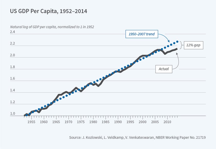
    Consider this: In 2006, before the financial crisis, were economists concerned with financial stability, bank runs, and systemic risk? Mostly not. Yet afterward, though banks are safer and risk is more tightly regulated, the knowledge that such possibilities are real has influenced research for more than a decade. Similarly, the knowledge that firms can suffer severe negative capital returns influences the actions and risks that firms are willing to take. Seeing the United States at the brink of financial collapse taught us that a financial crisis is more likely than we thought. The fact that firms have not seen another financial crisis in the last 10 years does not undermine that lesson. It is perfectly consistent with financial crisis being a once-in-50-years event. Even if no more crises are observed for the next 50 years, our estimate of this rare-event probability will still be informed by the 2008 event. In my research with Julian Kozlowski and Venky Venkateswaran, we explore this scarring effect as an explanation for the slow rebound of investment, labor, and output, as well as tail risk-sensitive options prices.¹

    While logical, this effect could be tiny. To assess whether this is a plausible explanation for the persistence of the post-crisis output loss, we embed learning in a dynamic stochastic general equilibrium model. For our purposes, this model needs two features. First, it needs to have shocks that had extreme (tail) outcomes in the financial crisis. Second, the model needs enough non-linearity so that unlikely tail events can have some aggregate effect. For this purpose, we use an augmented version of a model developed by François Gourio.² In this model, shocks have large initial effects, but there is no guarantee of any persistent effects from transitory shocks.

    The predictions of this model teach us some new lessons. First, the change in beliefs is large enough to make the drop in output a highly persistent level effect. This doesn't mean that the positive shocks in recent years cannot return the economy to trend. It does mean that, without the Great Recession, incomes today would have been higher. Second, the equilibrium effects are surprising. Some economists asserted that persistent economic responses to the Great Recession could not be due to tail risk because high tail risk would imply wide credit spreads and low equity prices. This logic would be correct if firms did not respond to higher risk by reducing their debt. But when risk and the price of credit both rise, firms demand less credit. They deleverage. Less indebted firms are less risky. As a result, their credit spread narrows and their equity price rebounds. Because of these competing forces, equity prices and interest rates are not reliable indicators of tail risk. However, the option prices offer a reliable measure of tail risk. Just as the Chicago Board Options Exchange's volatility index (VIX) measures option-implied volatility, the skewness index (SKEW) measures option-implied tail risk. After the Great Recession, the SKEW rose to record highs and never returned to its pre-crisis level.

Tail Risks, Low Interest Rates, and Inflation

    In follow-up work, we use a much simpler economic environment to speak to the persistently low interest rates on safe assets.³ To create a link between heightened tail risk and the interest rate, or yield, on safe assets, we focus on two standard mechanisms.

   First, faced with more risk, agents want to save more. But not every agent can save more. The bond market has to clear. Therefore, the return on bonds declines in order to clear that market. This force explains about a third of the decline in the interest rate. The second force at work is that safe assets offer liquidity that is particularly valuable in very bad conditions. When the probability of these tail events rises, liquid assets are more valuable and their yield declines, clearing the market. That liquidity effect explains the other two-thirds of the persistent interest rate gap from the pre-crisis period.

    If re-estimating distributions with real-time data can make actions persistently different following a crisis, does it matter how we estimate those distributions? For some purposes, no. For others, yes. In the secular stagnation paper, the magnitude of stagnation depended on the size of the increase in tail risk. That measurement is robust to many estimation methods. They all produce about the same effect, because they all fit the data by putting the same probability mass on extreme outcomes. Our agents used classical, non-parametric econometrics to estimate the shock distribution. We adopted this approach for its simplicity. Simplicity was essential because of the non-linearity and computational complexity of our economic framework. What doesn't work is a normal or thin-tailed distribution. It rules out any tail risk by construction.

    The choice of whether to use a Bayesian or classical estimator is not innocuous for all purposes. For example, in the presence of tail risk, finite-sample Bayesian estimators are biased.⁴ This bias arises because agents are confident that high inflation is more likely than extreme deflation. But they have few high-inflation data points with which to estimate that probability. The probability of high inflation could be much higher than they think. But it can't be much lower and a probability can't be below zero.

    Hassan Afrouzi, Michael Johannes, and I use this mechanism to understand why households, firms, and forecasters consistently report inflation forecasts with large positive bias.⁵ People seem to think inflation will be much higher than it turns out to be, month after month, year after year. These biases are shared by financial market participants who pay too much for inflation insurance relative to insurance on other risks.

    If a perfectly rational, Bayesian forecaster observes the time series of US inflation monthly from 1948 through 2018 and uses it to estimate a three-state mixture of normals, the estimated distribution has positive skewness of 0.38, and the average 2010–18 forecast is 1.45 percent higher than the average 2010–18 inflation realization. This is on par with the average size of the forecast bias from the University of Michigan Consumer Sentiment Index. If firms and forecasters observe additional data that are informative about inflation, the lower uncertainty reduces their inflation biases.

Estimating Changes in Tail Risk

    A final reason that the procedure for estimating beliefs matters is that estimating parameters that govern tail risk can make tail risk assessments and uncertainty quite volatile. With a non-parametric estimator, changes to a distribution are local: Each new data point affects the probability distribution by adding probability mass locally around the observed outcome and subtracting a small probability everywhere else. But with parametric systems, an observation in one part of the distribution can change a parameter estimate that significantly alters the probability mass elsewhere. In other words, observing ordinary, non-outlier events can affect our assessment of tail risk.

    Why are tail risk probabilities likely to be affected by observing nonlocal events? Because data on tail events are scarce, tail probability estimates are uncertain. Uncertain estimates are more likely to experience large revisions. In a parametric system, if there is a parameter that largely governs tail risk, that parameter will be tough to estimate with a high degree of confidence. For example, skewness is notoriously difficult to estimate. Observations not too far from the mean can nudge the estimate of a skewness parameter up or down. But a small change in skewness can double or triple the probability estimate of an outcome far out in the tail of a distribution.

    Such small adjustments in tail risk could be the origin of excess volatility or many apparent overreactions. Nicholas Kozeniauskas, Anna Orlik and I explore tail risk as a source of uncertainty shocks.⁶, ⁷ Uncertainty shocks have been a popular way of generating aggregate fluctuations in macroeconomic models, but it is not clear where they come from. Somehow, we pretend that everyone wakes up one day knowing for certain that the variance of some aggregate shock just rose. We do that because it helps explain aggregate phenomena, not because it makes sense. But one reason we might all suddenly feel uncertain is if we all observe an aggregate data point that makes disaster seem more likely than it was before.

    Using the post-war series of quarterly GDP growth, we apply Bayes' law to estimate parameters of a skewed distribution. Asking GDP to generate large swings in uncertainty is tough, because GDP is not a particularly volatile series. Yet when we allow agents to estimate a distribution that admits skewness, on average they estimate that GDP growth has a skewness coefficient of -0.3, which indicates that production meltdowns are more likely than "melt-ups." More importantly, the skewness estimate changes over time and it "wags the tail" of the distribution. Since tail events are far from the mean and uncertainty measures probability-weighted distance from the mean squared, these outliers move levels of uncertainty. We find that the standard deviation of the resulting uncertainty series is one-third of its average level. Those are large uncertainty fluctuations from a mundane macro time series.

    Macroeconomists have neglected tail risk, in part, because it is so difficult to measure. But the lack of data and difficulty of measurement are the things that make it interesting. Tail probability estimates are likely to diverge from true probabilities in ways that are persistent, volatile, and biased. All these econometric problems, and human faults, offer possible explanations for some of the most puzzling findings in aggregate economics.     Consider this: In 2006, before the financial crisis, were economists concerned with financial stability, bank runs, and systemic risk? Mostly not. Yet afterward, though banks are safer and risk is more tightly regulated, the knowledge that such possibilities are real has influenced research for more than a decade. Similarly, the knowledge that firms can suffer severe negative capital returns influences the actions and risks that firms are willing to take. Seeing the United States at the brink of financial collapse taught us that a financial crisis is more likely than we thought. The fact that firms have not seen another financial crisis in the last 10 years does not undermine that lesson. It is perfectly consistent with financial crisis being a once-in-50-years event. Even if no more crises are observed for the next 50 years, our estimate of this rare-event probability will still be informed by the 2008 event. In my research with Julian Kozlowski and Venky Venkateswaran, we explore this scarring effect as an explanation for the slow rebound of investment, labor, and output, as well as tail risk-sensitive options prices.¹

    While logical, this effect could be tiny. To assess whether this is a plausible explanation for the persistence of the post-crisis output loss, we embed learning in a dynamic stochastic general equilibrium model. For our purposes, this model needs two features. First, it needs to have shocks that had extreme (tail) outcomes in the financial crisis. Second, the model needs enough non-linearity so that unlikely tail events can have some aggregate effect. For this purpose, we use an augmented version of a model developed by François Gourio.² In this model, shocks have large initial effects, but there is no guarantee of any persistent effects from transitory shocks.

    The predictions of this model teach us some new lessons. First, the change in beliefs is large enough to make the drop in output a highly persistent level effect. This doesn't mean that the positive shocks in recent years cannot return the economy to trend. It does mean that, without the Great Recession, incomes today would have been higher. Second, the equilibrium effects are surprising. Some economists asserted that persistent economic responses to the Great Recession could not be due to tail risk because high tail risk would imply wide credit spreads and low equity prices. This logic would be correct if firms did not respond to higher risk by reducing their debt. But when risk and the price of credit both rise, firms demand less credit. They deleverage. Less indebted firms are less risky. As a result, their credit spread narrows and their equity price rebounds. Because of these competing forces, equity prices and interest rates are not reliable indicators of tail risk. However, the option prices offer a reliable measure of tail risk. Just as the Chicago Board Options Exchange's volatility index (VIX) measures option-implied volatility, the skewness index (SKEW) measures option-implied tail risk. After the Great Recession, the SKEW rose to record highs and never returned to its pre-crisis level.

Tail Risks, Low Interest Rates, and Inflation

    In follow-up work, we use a much simpler economic environment to speak to the persistently low interest rates on safe assets.³ To create a link between heightened tail risk and the interest rate, or yield, on safe assets, we focus on two standard mechanisms.

    First, faced with more risk, agents want to save more. But not every agent can save more. The bond market has to clear. Therefore, the return on bonds declines in order to clear that market. This force explains about a third of the decline in the interest rate. The second force at work is that safe assets offer liquidity that is particularly valuable in very bad conditions. When the probability of these tail events rises, liquid assets are more valuable and their yield declines, clearing the market. That liquidity effect explains the other two-thirds of the persistent interest rate gap from the pre-crisis period.

    If re-estimating distributions with real-time data can make actions persistently different following a crisis, does it matter how we estimate those distributions? For some purposes, no. For others, yes. In the secular stagnation paper, the magnitude of stagnation depended on the size of the increase in tail risk. That measurement is robust to many estimation methods. They all produce about the same effect, because they all fit the data by putting the same probability mass on extreme outcomes. Our agents used classical, non-parametric econometrics to estimate the shock distribution. We adopted this approach for its simplicity. Simplicity was essential because of the non-linearity and computational complexity of our economic framework. What doesn't work is a normal or thin-tailed distribution. It rules out any tail risk by construction.

    The choice of whether to use a Bayesian or classical estimator is not innocuous for all purposes. For example, in the presence of tail risk, finite-sample Bayesian estimators are biased.⁴ This bias arises because agents are confident that high inflation is more likely than extreme deflation. But they have few high-inflation data points with which to estimate that probability. The probability of high inflation could be much higher than they think. But it can't be much lower and a probability can't be below zero.

    Hassan Afrouzi, Michael Johannes, and I use this mechanism to understand why households, firms, and forecasters consistently report inflation forecasts with large positive bias.⁵ People seem to think inflation will be much higher than it turns out to be, month after month, year after year. These biases are shared by financial market participants who pay too much for inflation insurance relative to insurance on other risks.

    If a perfectly rational, Bayesian forecaster observes the time series of US inflation monthly from 1948 through 2018 and uses it to estimate a three-state mixture of normals, the estimated distribution has positive skewness of 0.38, and the average 2010–18 forecast is 1.45 percent higher than the average 2010–18 inflation realization. This is on par with the average size of the forecast bias from the University of Michigan Consumer Sentiment Index. If firms and forecasters observe additional data that are informative about inflation, the lower uncertainty reduces their inflation biases.

Estimating Changes in Tail Risk

    A final reason that the procedure for estimating beliefs matters is that estimating parameters that govern tail risk can make tail risk assessments and uncertainty quite volatile. With a non-parametric estimator, changes to a distribution are local: Each new data point affects the probability distribution by adding probability mass locally around the observed outcome and subtracting a small probability everywhere else. But with parametric systems, an observation in one part of the distribution can change a parameter estimate that significantly alters the probability mass elsewhere. In other words, observing ordinary, non-outlier events can affect our assessment of tail risk.

    Why are tail risk probabilities likely to be affected by observing nonlocal events? Because data on tail events are scarce, tail probability estimates are uncertain. Uncertain estimates are more likely to experience large revisions. In a parametric system, if there is a parameter that largely governs tail risk, that parameter will be tough to estimate with a high degree of confidence. For example, skewness is notoriously difficult to estimate. Observations not too far from the mean can nudge the estimate of a skewness parameter up or down. But a small change in skewness can double or triple the probability estimate of an outcome far out in the tail of a distribution.

    Such small adjustments in tail risk could be the origin of excess volatility or many apparent overreactions. Nicholas Kozeniauskas, Anna Orlik and I explore tail risk as a source of uncertainty shocks.⁶, ⁷ Uncertainty shocks have been a popular way of generating aggregate fluctuations in macroeconomic models, but it is not clear where they come from. Somehow, we pretend that everyone wakes up one day knowing for certain that the variance of some aggregate shock just rose. We do that because it helps explain aggregate phenomena, not because it makes sense. But one reason we might all suddenly feel uncertain is if we all observe an aggregate data point that makes disaster seem more likely than it was before.

    Using the post-war series of quarterly GDP growth, we apply Bayes' law to estimate parameters of a skewed distribution. Asking GDP to generate large swings in uncertainty is tough, because GDP is not a particularly volatile series. Yet when we allow agents to estimate a distribution that admits skewness, on average they estimate that GDP growth has a skewness coefficient of -0.3, which indicates that production meltdowns are more likely than "melt-ups." More importantly, the skewness estimate changes over time and it "wags the tail" of the distribution. Since tail events are far from the mean and uncertainty measures probability-weighted distance from the mean squared, these outliers move levels of uncertainty. We find that the standard deviation of the resulting uncertainty series is one-third of its average level. Those are large uncertainty fluctuations from a mundane macro time series.

    Macroeconomists have neglected tail risk, in part, because it is so difficult to measure. But the lack of data and difficulty of measurement are the things that make it interesting. Tail probability estimates are likely to diverge from true probabilities in ways that are persistent, volatile, and biased. All these econometric problems, and human faults, offer possible explanations for some of the most puzzling findings in aggregate economics.