KALMAN

Options     Examples     References

KALMAN estimates linear models using the Kalman filter method. It can handle fairly general State Space models, but it is typically used to estimate regression-type models where the coefficients follow a random process over time.

KALMAN (BPRIOR=<prior vector>, BTRANS=<matrix of coefficients in transition equation>,

                EMEAS, ETRANS, PRINT, SILENT,SMOOTH, VBPRIOR=<variance of prior>,

                VMEAS=<variance factor in measurement equation>,

                VTRANS=<variance factor in transition equation>,

                XFIXED=<X matrix for measurement equation>)

                <list of dependent variables> [| <list of independent variables>];

Usage

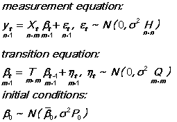
The Kalman filter model consists of two parts (the state space form):

The matrices T, H, and Q are assumed to be known, and they each default to the identity matrix if they are not supplied by the user in the KALMAN options list. Note that they are not allowed to vary over time, but this constraint can be easily relaxed by running KALMAN within a loop over the sample. The NOEMEAS and NOETRANS options are used to zero the variances of the measurement and transition equations respectively.

The y(t) and X(t) variables are the dependent and independent variables, just as in ordinary least squares. If you want to use more than one dependent variable, list all the y variables first, then a |, and then list the X variables for each y (duplicate the X list if they are the same for every y). You may want to insert zeros along with the X variables to prevent cross-equation restrictions (see the Examples). If X(t) is fixed over the sample, use the XFIXED option.

To get a time-varying parameter model, specify VTRANS=Q (the noise-to-signal ratio) and BTRANS=T (if it is not the identity matrix).

To evaluate the likelihood function for general ARMA(p,q) models, fill the BTRANS and VTRANS matrices with the estimated coefficients for the model; see Harvey, p.103 for the general form.

Output

A standard table of coefficients and standard errors is printed for the final state vector, along with the log likelihood. The following items are stored (and may be printed):

Note that the first few rows in the residuals or state vectors may be zero if those observations were used to calculate priors. Note also that recursive residuals for OLS regressions can be obtained using OLSQ with the following options set:

REGOPT (CALC) RECRES;  

Method

The Kalman filter recursively updates the estimate of beta(t) (and its variance), using the new information in y(t) and X(t) for each observation, so it can be viewed as a Bayesian method. However, the user does not have to supply priors; they are calculated automatically for regression-type models from the initial observations of the sample. See the Harvey reference for the actual updating formulas. If the default prior is singular, KALMAN adds one more observation to the calculation. The smoothed state vectors (if requested) are estimates based on the full sample; again, see Harvey for the details.

The method of estimation for each time period is maximum likelihood conditional on the data observed to that point. An orthonormalizing transformation of X is used to improve accuracy.

The variance sigma squared and the log likelihood are computed from the recursive residuals. The recursive residuals are

in Harvey's notation, so that E[e(t)'e(t)] = I. If you do not factor sigma squared out of H, Q, and P(0), the estimated @S2 should be close to unity. For m>1, if the prediction errors are collinear, there may be problems estimating sigma squared, the standard errors, recursive residuals, and log likelihood.

Options

BPRIOR= the vector of prior coefficients b(0) for measurement equation. Required if XFIXED is used; otherwise it will be calculated by default from a regression in the initial observations of the sample. If the first m observations are not sufficient to identify the prior, one observation is added and BPRIOR is estimated again.

BTRANS= T, the matrix of coefficients in the transition equation (default identity matrix).

EMEAS/NOEMEAS indicates the presence of an error term in the measurement equation (NOEMEAS or NOEM is the same as VMEAS = zero).

ETRANS/NOETRANS indicates the presence of an error term in the transition equation.

PRINT/NOPRINT prints the prior, @STATE, @RES1, @RECRES, @SMOOTH, @RESD.

SILENT/NOSILENT turns off most of the output.

SMOOTH/NOSMOOTH computes fixed-interval smoothed estimates of the state vector b(t) (stored in @SMOOTH) and the direct residuals @RESD.

VBPRIOR= P(0), the variance of the prior (symmetric matrix). Required if BPRIOR is specified. Note: sigma squared is factored out of this matrix.

VMEAS= H, the variance of the measurement equation (symmetric matrix). Default: identity matrix. In Harvey's notation, this is SHS'.

VTRANS= Q, the variance of the transition equation (symmetric matrix). Default: identity matrix. Specifies the "noise-to-signal ratio" if H = identity matrix. In Harvey's notation, this is RQR'.

XFIXED= X matrix for measurement equation, when it is fixed over time.

Examples

One of the simplest Kalman filter models is equivalent to OLSQ (using a transition equation of b(t) =b(t-1) =b). This model can be estimated with the command:

KALMAN (NOETRANS) Y C X;

which produces the same coefficient estimates as OLSQ Y C X ;, but calculates them recursively, along with the recursive residuals.

To estimate a Cooley-Prescott "adaptive regression" model where b(t) follows random walk with a nondiagonal variance matrix:

KALMAN (VTRANS=NSRMAT) Y C X1 X2;

A "stochastically convergent parameter" model (convergent towards zero in this case, since the transition matrix has roots less than one):

MFORM (TYPE=DIAG,NROW=3) TMAT=.9;

KALMAN (BTRANS=TMAT,VTRANS=NSRMAT) Y C X1 X2;

Here is an example with two dependent variables; note the two lists of exogenous variables, which must be of the same length. In this case, both equations are forced to have the same two coefficients.

KALMAN (NOET) Y1 Y2 | C1 X1, C2 X2;

The example below has two dependent variables, but in this case the equations have separate coefficients; note the use of zero variables. This specification is still somewhat unrealistic because H is identity (same variance and no correlation between errors in the equations):

ZERO = 0;

KALMAN (NOET) Y1 Y2 | C1 X1 ZERO ZERO, ZERO ZERO C2 X2;

Harvey's Example 2 (p.116-117) ("signal plus noise" or Cooley-Prescott):

READ Y; 4.4 4.0 3.5 4.6;

SET Q = 4; SET A0 = 4; SET P0 = 12;

KALMAN (VT=Q,BPRIOR=A0,VBPRIOR=P0) Y C;

Harvey's Exercise 1 (p.119) (stochastically convergent):

READ Y; 4.4 4.0 3.5 4.6;

Y4 = Y-4;

SET RHO=.5; SET Q = 4; SET A0 = .2; SET P0 = 3;

KALMAN (BT=RHO,VT=Q,BP=A0,VBP=P0) Y4 C;

Bootstrapping a variance for the transition equation:

SMPL 1,100;

KALMAN (NOETRANS) Y C X1 X2;

UNMAKE @STATE B1-B3;

SMPL 4,100;

DOT 1-3;

     D.=B.-B.(-1);

ENDDOT;

COVA D1-D3;

MAT VTOS=@COVA/@S2;

KALMAN  (VTRANS=VTOS) Y C X1 X2;

Hyperparameter estimation using ML PROC. This example estimates the variances of the transition matrix Q, using the ML PROC.

MFORM(NROW=2,TYPE=SYM) Q;

PARAM Q11,1 Q22,2;

ML KFQ Q11,Q22;

? KFQ evaluates log likelihood for ML PROC

PROC KFQ;

     IF (Q11<=0 .OR. Q22<=0); THEN; ? Check constraints

          SET @LOGL=@MISS;               ? Are variances >0?

     ELSE; DO;                                          ? yes, evaluate.

          SET Q(1,1) = Q11; SET Q(2,2) = Q22;

          SUPRES @COEF;

          KALMAN(SILENT,VTRANS=Q) Y C X;

          NOSUPRES @COEF;

     ENDDO;

ENDPROC;

References

Cooley, T. F. and Edward Prescott, "Varying Parameter Regression: A Theory and Some Applications," Annals of Economic and Social Measurement 2 (1973), pp. 463-474.

Cooper, J. Philip, "Time-Varying Regression Coefficients: A Mixed Estimation Approach and Operational Limitation of the General Markov Structure," Annals of Economic and Social Measurement 2(1973), pp. 525-530.

Harvey, Andrew C., Time Series Models, 1981, Philip Allen, London, pp.101-119.

Harvey, Andrew C., Forecasting, Structural Time Series Models and the Kalman Filter, 1989, Cambridge University Press, New York.

Kalman, R. E., “A New Approach to Linear Filtering and Prediction Problems,” Journal of Basic Engineering, Transactions ASME, Series D 82 (1960): 35-45.

Maddala, G. S., Econometrics, 1977, McGraw-Hill Book Co., New York, pp.396-400.