ARCH estimates regression models with AutoRegressive Conditional Heteroskedasticity (originated by Robert Engle). It will estimate any model from linear regression to GARCH-M. ARCH models allow the residuals to have a variable variance (but still have zero conditional mean) over the sample. This contrasts with AR(1) models or general transfer function models where the residuals do not have zero conditional mean. ARCH models are often used to model exchange rate fluctuations and stock market returns.
ARCH (E2INIT=method, GT=<list of weighting series>, HEXP=<value of lambda>,
HINIT=method, MEAN, NAR=<number of AR terms for regular ARCH>,
NMA=<number of MA terms for GARCH>, RELAX, ZERO, nonlinear options)
<dependent variable> [<list of independent variables>];
Usage
The ARCH command is just like the OLSQ command, except for the options which model the heteroskedasticity of the residuals. The default model estimated if no options are included is GARCH(1,1).
Method
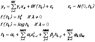
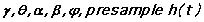
The generalized form of ARCH (GARCH-M) estimated by TSP is given by the following equations (see McCurdy and Morgan):
An immediate issue is the identification of the order of the ARCH or GARCH process. Bollerslev suggests obtaining squared residuals from OLS and using standard Box-Jenkins techniques (BJIDENT in TSP) on these squared residuals. It is also possible to estimate several ARCH models and use likelihood ratio tests to determine the proper specification.
All models are estimated by maximum likelihood (normally with analytic first and second derivatives). Presample values of h and the disturbance epsilon are initialized by the methods specified in the HINIT and E2INIT options.
ARCH will not work if there are gaps in the SMPL -- instead, it is possible to use dummy variables (as right hand side variables and in GT= ) to exclude observations from the fit.
Default starting values for gamma are obtained from the OLS slope coefficients, while a(0) and presample h(t) (if HINIT=ESTALL is used) are started from the OLS ML estimate of the variance of the disturbance. Other parameters are initialized to 0. These defaults apply to all models except when NAR=0 and NMA>0, in which case a(0)=0 and b(1)=1 are used (to prevent false convergence to the OLS saddlepoint solution). The defaults may be overridden if an @START vector is provided by the user (with a value for each parameter -- see the final example below).
Several constraints are imposed on the ARCH parameters to protect against numerical problems from negative, zero, or infinite variances:
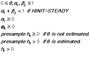
Use of the ZERO/NOZERO option controls the technique for bounding (see the description under Options below). If a parameter is bounded on convergence, its standard error is set to zero to make the other estimates conditional on it. In this case, it is wise to try some alternative non-bounded starting values to check for an interior ML solution (see the final example).
Output
A title is printed, based on the options, indicating OLS, OLS-W, OLS-M, ARCH, ARCH-M, GARCH, or GARCH-M estimation. Standard iteration output follows with starting values, etc. Then standard regression output is printed; the only difference is the extra coefficients. The order of the estimated coefficients is:
h(t) is stored in @HT.
E2INIT=HINIT or INDATA or PREDATA specifies the initialization of the presample values of epsilon. The default HINIT sets them equal to h(t) (their unconditional expectation, as given by the current HINIT option). INDATA reserves the first NAR observations in the current sample to compute residuals and squares these (this was the default in TSP Version 4.3 and earlier). PREDATA attempts to use NAR observations prior to the current sample to compute such squared residuals (if such observations are missing, some observations from the current sample are used).
GT= a list of weighting series g(k,t). The estimated coefficients for these series are labeled as PHI_series1, PHI_series2, etc. in the output. Note that the constant C should not be in the GT list because it is already included in h(t) via a(0). If GT is used without NAR or NMA, the model is called OLS-W or OLS-M by TSP. Use the RELAX option to relax the constraint on phi.
HEXP= value of the exponent of the conditional variance h(t) in the regression equation. The default value of HEXP is 0.5, which means that the disturbance depends on the standard deviation of its distribution.
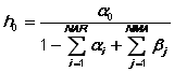
HINIT=ESTALL or OLS or SSR or STEADY or value specifies the initialization of the presample values of ht . ESTALL estimates them as nuisance parameters (labelled H(0), H(-1), etc.); this was the default in TSP Version 4.3 and earlier. OLS holds them fixed at the initial ML estimate of the residual variance from OLS. The default SSR sets them equal to SSR/T, where SSR is the sum of squared residuals from the current parameter values (see Fiorentini et al (1996)). STEADY sets them equal to their steady state value
Note that the denominator must be strictly positive, and that the expectation of phi(k)g(k,t) is assumed to be zero. The user may also specify an arbitrary fixed value .
MEAN/NOMEAN controls whether the theta f(h,t) term appears in the regression. This is labelled THETA in the output. MEAN indicates a GARCH-M, ARCH-M, or OLS-M model, and the GT, NAR, or NMA options are required. The constraints on theta can be relaxed if necessary by using the RELAX option. See the HEXP option.
NMA= the number of terms where h(t) depends on its past values. These coefficients are labelled BETA1, BETA2, etc. in the output. This indicates a GARCH model.
NAR= the number of terms where h(t) depends on past squared residuals. These coefficients are labelled ALPHA1, ALPHA2, etc. in the output. This indicates a pure ARCH model if NMA=0.
RELAX/NORELAX relaxes the constraints on theta and phi.
ZERO/NOZERO specifies the method of imposing constraints on the parameters. If the default ZERO option is used, a parameter is set equal to the bound if the trial value violates the bound. Note that ZERO does not apply to parameters with strict inequality constraints, such as h(t). With NOZERO, the stepsize is squeezed when the bound is violated (until the constraint is met). NOZERO appears to be much slower than ZERO.
Nonlinear options These options control the iteration methods and printing. They are explained in the NONLINEAR section of this manual. Some of the common options are MAXIT, MAXSQZ, PRINT/NOPRINT, and SILENT/NOSILENT.
The default Hessian choices are HITER=N and HCOV=W . Other choices like B, F, and D are also legal, but Fiorentini et al (1996) show that HITER=N results in fast convergence, and HCOV=W yields standard errors that are robust to non-normal disturbances.
If no options are supplied, a GARCH(1,1) model will be estimated.
ARCH(NAR=4) Y C X; ? Pure ARCH
ARCH Y C X; ? GARCH(1,1) (the default)
ARCH(NMA=1,NAR=3,MEAN) Y C X; ? GARCH-M
ARCH(GT=(G1,G2,G3),MEAN) Y C X; ? OLS-M
GARCH(0,1): Here we try some alternative starting values to override the solution with beta1=1 that can occur in these models. The order of parameters in @COEF and @START is described below under Output -- the first 3 parameters are the gammas and the last 3 are alpha0, beta1, and h(0).
ARCH(NMA=1) DF C DF2 MHOL;
COPY @COEF @START;
SET @START(4) = .02; ?ALPHA0
SET @START(5) = .5; ?BETA1
ARCH(NMA=1) DF C DF2 MHOL;
Other types of univariate and multivariate GARCH models can be estimated with ML and ML PROC. Please see the TSP User's Guide and our web page http://www.tspintl.com for examples.
Bollerslev, Tim, "Generalized Autoregressive Conditional Heteroscedasticity," Journal of Econometrics 31 (1986), pp.307-327.
Engle, Robert F., "Autoregressive Conditional Heteroscedasticity with Estimates of the Variance of U.K. Inflation," Econometrica 50 (1982), pp.987-1007.
Engle, Robert F., David M. Lilien, and Russell P. Robins, Estimating Time Varying Risk Premia in the Term Structure: The ARCH M Model, Econometrica 55(1987), pp. 391 407.
Fiorentini, Gabriele, Calzolari, Giorgio, and Panattoni, Lorenzo, "Analytic Derivatives and the Computation of GARCH Estimates," Journal of Applied Econometrics 11 (1996), pp.399-417.
McCurdy, Thomas H., and Morgan, Ieuan G., "Testing the Martingale Hypothesis in Deutsche Mark Futures with Models Specifying the Form of Heteroscedasticity," Journal of Applied Econometrics 3 (1988), pp.187-202.